循环神经网络RNN(示例代码LSTM预测股价示例)
1 应用场景:
AI翻译,AI对话,股票预测,行为判断
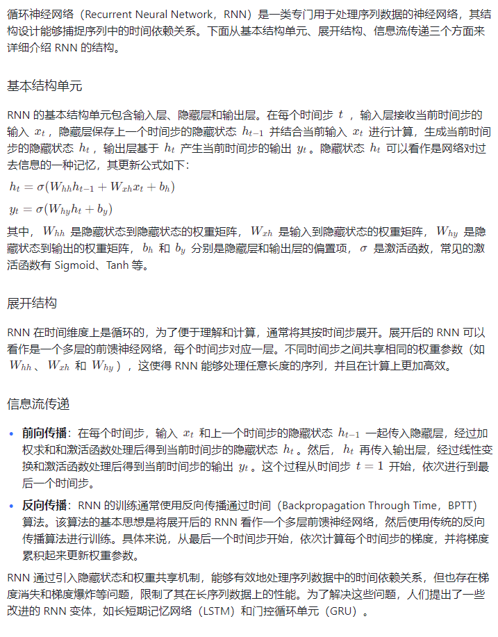
2 背景介绍
3 代码:
import pandas as pd
import numpy as np
import baostock as bs#下载数据
def get_stock_data_and_save_to_csv(stock_code, start_date, end_date, file_path):# 登陆系统lg = bs.login()if lg.error_code != '0':print(f"登录失败,错误代码: {lg.error_code},错误信息: {lg.error_msg}")return# 获取股票数据rs = bs.query_history_k_data_plus(stock_code,"date,code,open,high,low,close,preclose,volume,amount,adjustflag,turn,tradestatus,pctChg,peTTM,pbMRQ,psTTM,pcfNcfTTM,isST",start_date=start_date, end_date=end_date,frequency="d", adjustflag="3")if rs.error_code != '0':print(f"获取数据失败,错误代码: {rs.error_code},错误信息: {rs.error_msg}")bs.logout()return# 打印结果集data_list = []while (rs.error_code == '0') & rs.next():# 获取一条记录,将记录合并在一起data_list.append(rs.get_row_data())result = pd.DataFrame(data_list, columns=rs.fields)try:# 保存到CSV文件result.to_csv(file_path, index=False)print(f"数据已成功保存到 {file_path}")except Exception as e:print(f"保存数据到文件时出错: {e}")# 登出系统bs.logout()if __name__ == "__main__":stock_code = "sh.603236"start_date = "2024-08-22"end_date = "2025-08-22"file_path = "stock_data_603236_short.csv"get_stock_data_and_save_to_csv(stock_code, start_date, end_date, file_path)
%matplotlib inline
from matplotlib import pyplot as plt
fig1 = plt.figure(figsize=(8,5))
plt.plot(price)
plt.title('close price')
plt.xlabel('time')
plt.ylabel('price')
plt.show()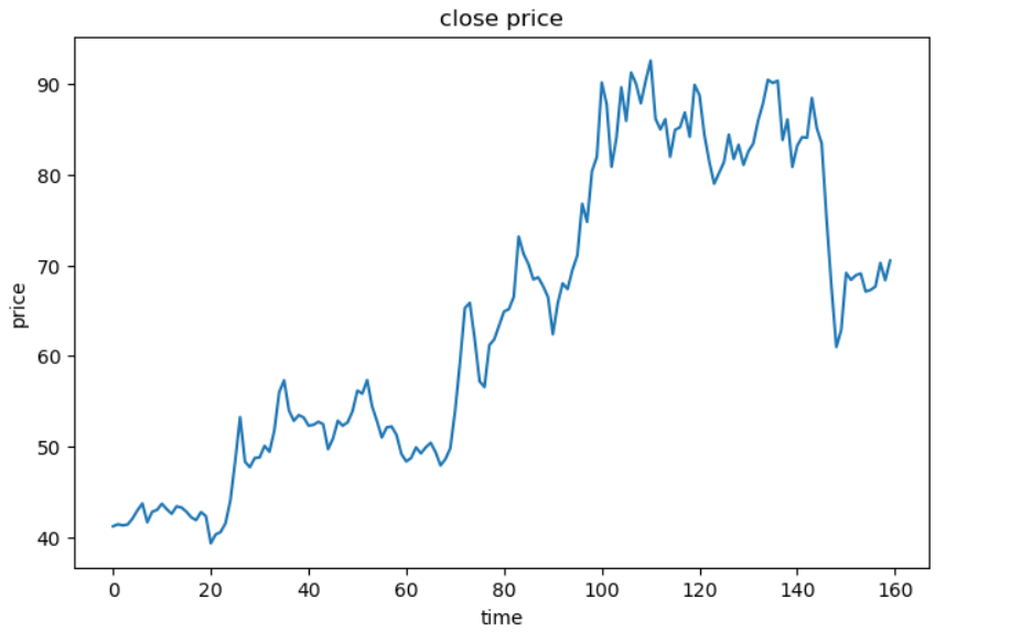
# define X and y
# define method to extract X and y
def extract_data(data, time_step):X=[]y=[]for i in range(len(data)-time_step):X.append([a for a in data[i:i+time_step]])y.append(data[i+time_step])X = np.array(X)X = X.reshape(X.shape[0], X.shape[1], 1)return X, y#define X and y
time_step = 8
X,y = extract_data(price_norm, time_step)
print(X[0,:,:])
print(y)
print(X.shape, len(y))
#set up the model
from keras.models import Sequential
from keras.layers import Dense, SimpleRNN
model = Sequential()
#add RNN layer
model.add(SimpleRNN(units=5,input_shape=(time_step,1), activation='relu'))
#add output layer
model.add(Dense(units=1,activation='linear'))
#configure the model
model.compile(optimizer='adam', loss = 'mean_squared_error')
model.summary()
#train the model
y = np.array(y)
model.fit(X,y,batch_size=30, epochs=200)
#make prediction base on the traing data
y_train_predict = model.predict(X)*max(price)
y_train = y*max(price)
print(y_train_predict, y_train)
%matplotlib inline
from matplotlib import pyplot as plt
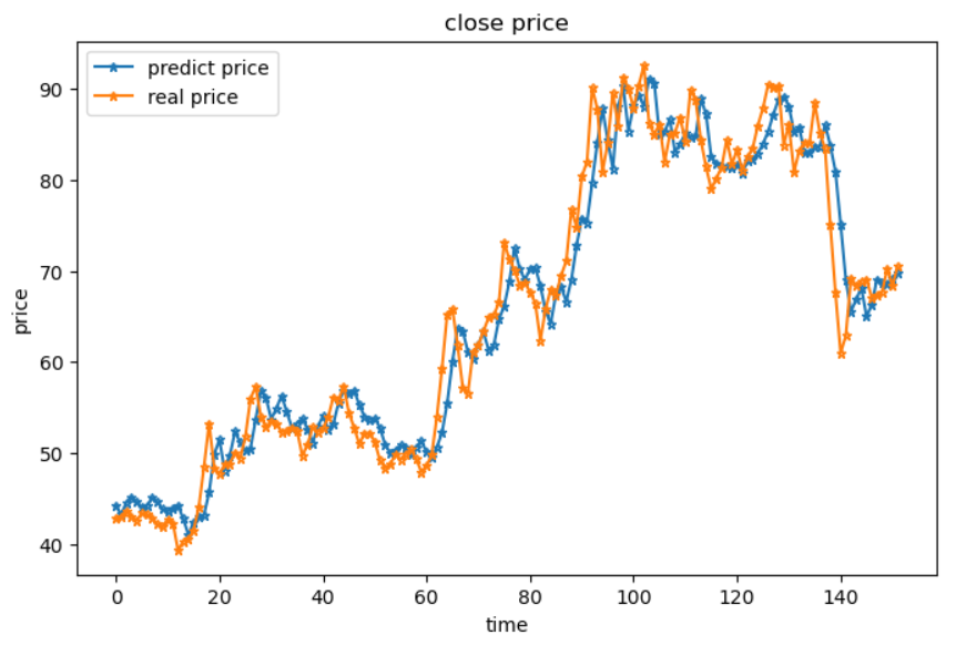
fig2 = plt.figure(figsize=(8,5))
plt.plot(y_train_predict, label = 'predict price',marker='*', markersize=5,markerfacecolor='none')
plt.plot(y_train, label = 'real price',marker='*', markersize=5,markerfacecolor='none')
plt.title('close price')
plt.xlabel('time')
plt.ylabel('price')
plt.legend()
plt.show()