Python数据分析案例72——基于股吧评论数据的情感分析和主题建模(LDA)
背景
好久没更新了,最近忙其他去了。最近股市波动太大,看了不少新闻的评论。抽空写了个股吧评论数据的LDA建模和情感分析,简单写到博客上来更新一下。
数据来源
上证指数(000001)股吧_上证指数怎么样_分析讨论社区—
数据来源上述网站的东方财富网,对于指数的评论。股吧评论:
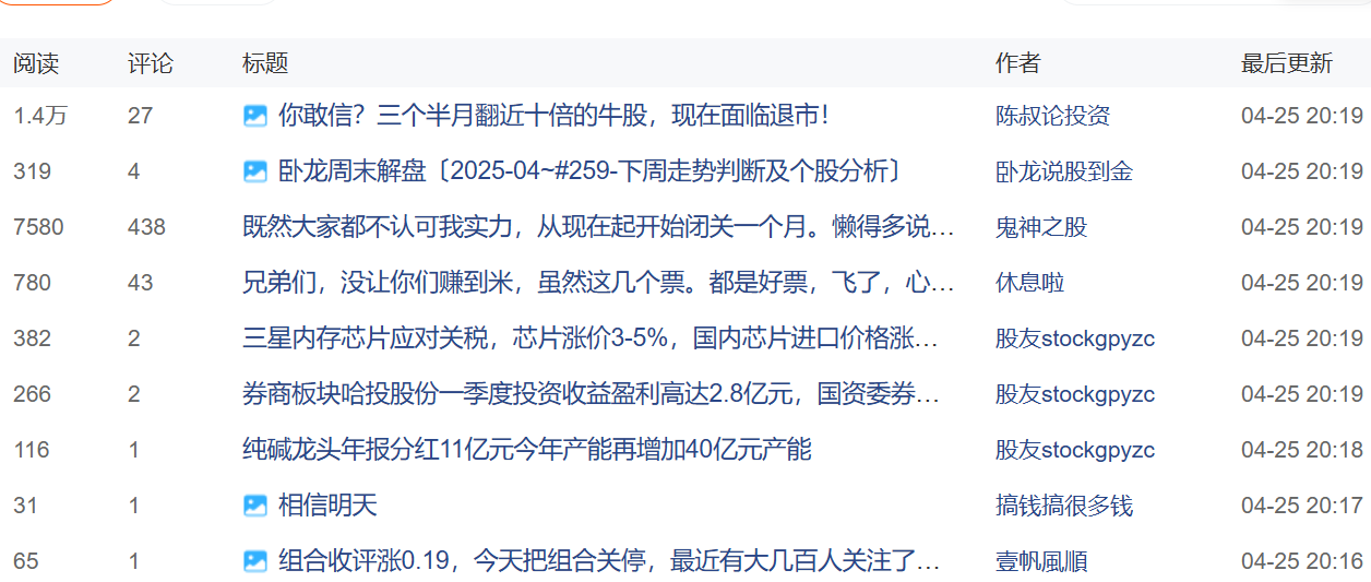
这次就没用python代码去爬虫,直接使用浏览器的插件(Instant Data Scraper)进行数据的获取,还是很便捷的,懒得写代码了,就直接用插件爬下来存为csv文件进行分析。数据量还有点大,我本来想爬取2个月的,但是一天的量就有2k多条,所以就只爬取了一个星期。:
数据量2.6w多条。从4-13号上午到4-21号上午。
当然,本次案例的数据和全部代码文件还是可以参考:股吧评论LDA
代码实现
读取数据
数据分析第一步,导入包
import pandas as pd
import numpy as np
import matplotlib.pyplot as plt
import seaborn as sns
import jieba , re
from collections import Counter
from snownlp import SnowNLP
from wordcloud import WordCloudplt.rcParams['font.sans-serif'] = ['KaiTi']  #指定默认字体
plt.rcParams['axes.unicode_minus'] = False   #解决保存图像是负号
读取数据,展示前五行
df = pd.read_excel('股吧评论文本.xlsx')
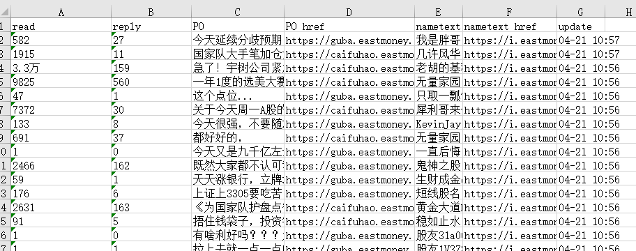
df.head()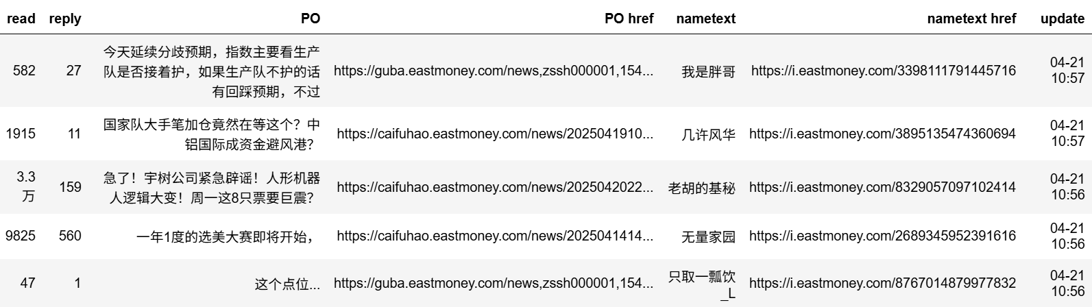
可以看到,数据总共有七列,从左到右分别是阅读量,回复量。评论内容,评论链接,用户名,用户链接以及评论时间。查看数据信息
df.info()
数据没有缺失值。
数据清洗
由于数据的阅读量里面有“万”这种字符串,需要进行一定的预处理
def check_万(txt):if '万' in txt:txt=txt.replace('万','')number=int(float(txt)*10000)else:number=int(float(txt))return numberapply向量化处理这一列。
## 数值处理
df['阅读量']=df['read'].apply(check_万)
时间列进行处理,加上年份,转为时间格式
# 时间处理
df['时间'] = pd.to_datetime('2025-' + df['update'], format='%Y-%m-%d %H:%M')
## 重命名,选择需要的列
df=df.rename(columns={'PO':'评论文本' ,'nametext':'用户名','reply':'回复量'})[['时间','评论文本','用户名','阅读量','回复量']].set_index('时间').sort_index()
df.head()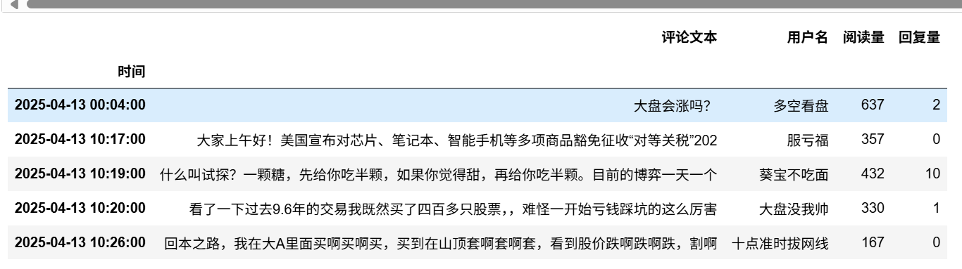
数据整理好了。第一列是时间索引,后面是评论,用户名,阅读量,回复量。
然后我们要使用SnowNLP库进行情感标记吗,这个库可以对一个中文文本标记其情感数值,取值为0是完全富负面情感,取值=1是完全正面情感。
### 情感值计算
df['情感值'] = df['评论文本'].apply(lambda x: SnowNLP(x).sentiments)
df['评论文本长度']=df['评论文本'].apply(lambda x: len(x))
新增两列,一列是情感值,一列是评论文本长度。
可以把预处理完后的数据存储一下:
df.to_excel('清洗完成数据.xlsx')
基础性分析
读取
df=pd.read_excel('清洗完成数据.xlsx',parse_dates=['时间']).set_index('时间')查看不同天的评论数量可视化
df.index.day.value_counts().sort_index().plot(figsize=(8,3),title='不同日期的评论数量')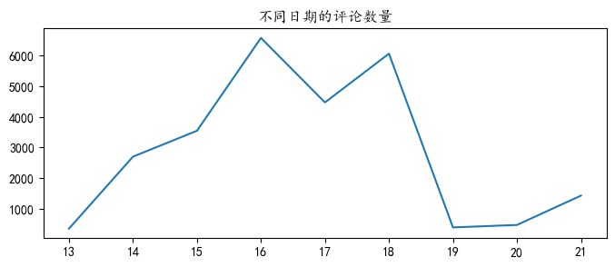
可以看到15-18号的文本评论数量较多,13,14,20,21是周末,不开盘,所以股吧评论很少。
查看不同时间段的文本数量
df.index.hour.value_counts().sort_index().plot.pie(figsize=(5,5),title='不同时间段的评论数量')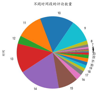
可以看到从9点开始评论逐渐变多,12点较少,因为中午休息。13,14点的评论最多,15点收盘后评论又开始变少。
查看评论的文本长度和情感值的数值型的分布:
# 设置画布和子图
fig, axes = plt.subplots(2, 1, figsize=(5,4), dpi=168)# 为每个变量绘制核密度图
sns.histplot(ax=axes[0], data=df['评论文本长度'], fill=True)
axes[0].set_title('评论文本长度直方图')
axes[0].tick_params(axis='x', labelsize=7, rotation=0)
axes[0].set_xlabel('')
sns.histplot(ax=axes[1], data=df['情感值'],fill=True)
axes[1].set_title('文本情感值核直方图')
axes[1].tick_params(axis='x', labelsize=7, rotation=0)
axes[1].set_xlabel('')
# 调整子图间距
plt.tight_layout()# 显示图表
plt.show()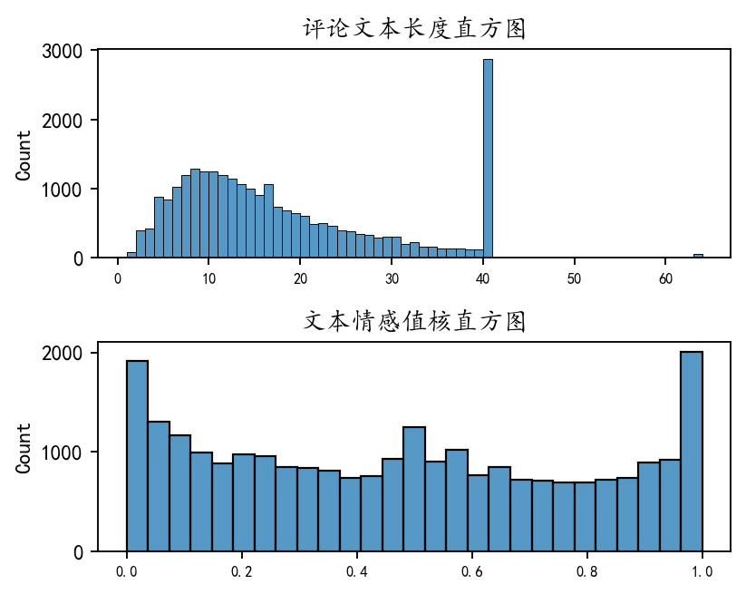
可以看到评论文本的长度是一个右偏分布,具有很多极大值,大部分评论长度在10附近,所以股吧的评论都是短评。
文本情感值的分布是一个中间密度偏少。两边密度偏高的分布,也就是说很多评论较为极端,要么是极其的正向,要么极其的负向,中间比较中性的评论偏少。
查看阅读量和回复量的分布:
# 设置画布
plt.figure(figsize=(10, 4), dpi=128)# 第一个子图(阅读量)
plt.subplot(1, 2, 1)
plt.boxplot(df['阅读量'], patch_artist=True, boxprops=dict(facecolor='skyblue'))
plt.yscale('log')  # y轴对数化(箱线图一般y轴是数值)
plt.title('阅读量 (log scale)')
plt.ylabel('数值(对数)', fontsize=8)
plt.xticks([1], ['阅读量'], fontsize=8)  # 设置x轴标签# 第二个子图(回复量)
plt.subplot(1, 2, 2)
plt.boxplot(df['回复量'], patch_artist=True, boxprops=dict(facecolor='salmon'))
plt.yscale('log')  # y轴对数化
plt.title('回复量 (log scale)')
plt.ylabel('数值(对数)', fontsize=8)
plt.xticks([1], ['回复量'], fontsize=8)  # 设置x轴标签# 调整子图间距
plt.tight_layout()# 显示图表
plt.show()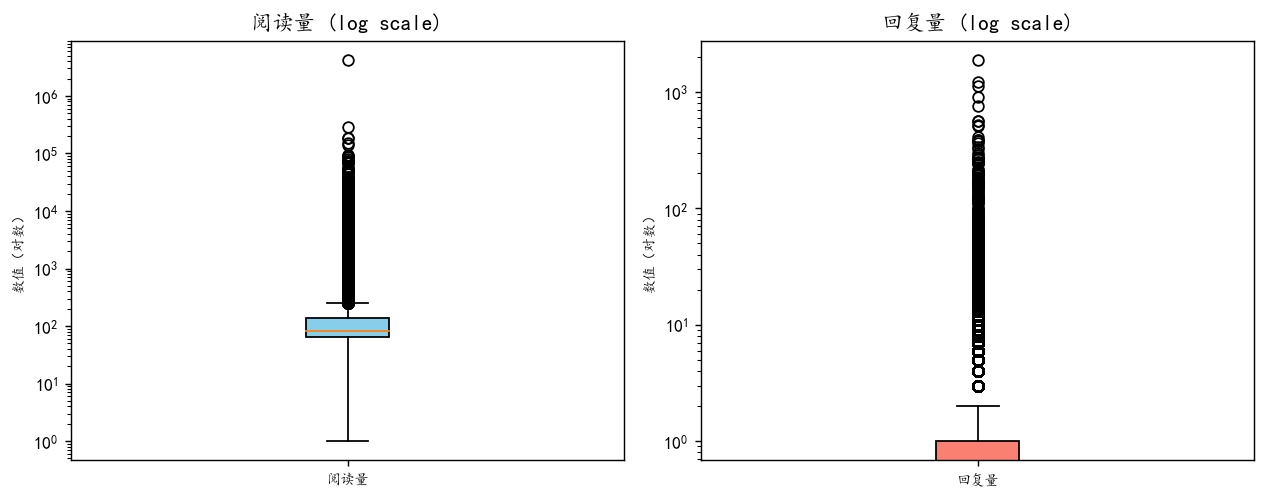
可以看到也是很严重的右偏分布,很多极大值。说明只有少数的评论会收到较多的阅读和回复。
分组聚合
下面进行分组聚合,查看不同日期的、小时时间段的 情感值
新增两列
df['日期号']=df.index.day
df['小时']=df.index.hour
画出每日情感值均值的柱状图:
daily_sentiment = df.groupby('日期号')['情感值'].mean().reset_index()# 设置画布
plt.figure(figsize=(7, 3),dpi=128)
# 使用 seaborn 绘制柱状图,颜色使用 HUSL 调色板
sns.barplot( data=daily_sentiment,  x='日期号',  y='情感值',palette='husl',  # 使用 HUSL 颜色edgecolor='black',  # 边框颜色linewidth=0.5,  # 边框线宽
)# 优化图表
plt.title('每日情感均值')
plt.xlabel('日期号')
plt.ylabel('平均情感值')
#plt.xticks(rotation=45)  # 旋转 x 轴标签避免重叠
plt.tight_layout()  # 自动调整布局
plt.show()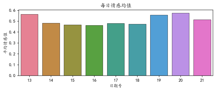
可以看到14-19号工作日,开盘的时候评论的平均情感值是偏低的。说明股市开盘的日子人们会发出负面的评论。
画出不同的小时的情感值均值的柱状图:
hour_sentiment = df.groupby('小时')['情感值'].mean().reset_index()# 设置画布
plt.figure(figsize=(7, 3),dpi=128)
# 使用 seaborn 绘制柱状图,颜色使用 HUSL 调色板
sns.barplot( data=hour_sentiment,  x='小时',  y='情感值',palette='husl',  # 使用 HUSL 颜色edgecolor='black',  # 边框颜色linewidth=0.5,  # 边框线宽
)# 优化图表
plt.title('不同时间段情感均值')
plt.xlabel('小时')
plt.ylabel('平均情感值')
#plt.xticks(rotation=45)  # 旋转 x 轴标签避免重叠
plt.tight_layout()  # 自动调整布局
plt.show()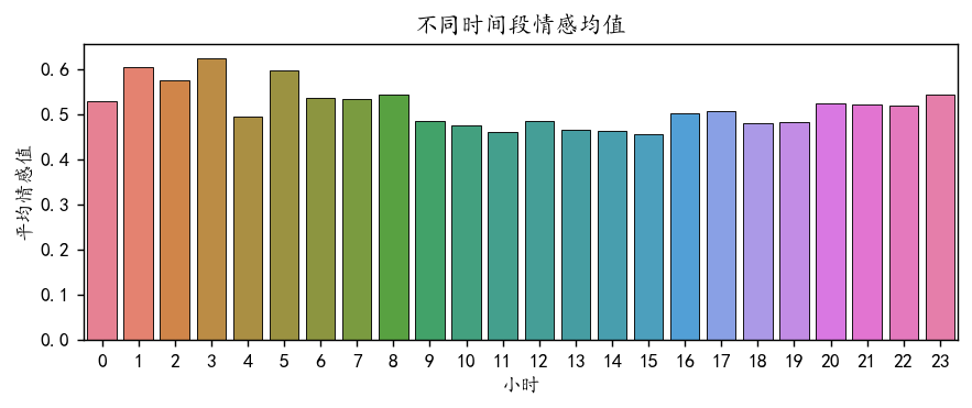
可以看到9-15点的情感值明显要低一些,也就是说,股市开盘的日子人们会更加倾向发出负面的评论。
文本分析
文本分词
中文文本需要进行分词处理,然后过滤掉一些不常用的停用词。
# 读取停用词文件,创建停用词列表
stop_words = []
with open('停用词.txt', 'r', encoding='utf-8') as file:stop_words = [line.strip() for line in file]
stop_words[:3]
# 定义分词和停用词过滤函数
def txt_cut(juzi):return " ".join([w for w in jieba.lcut(juzi) if w not in stop_words and not re.search(r'\d', w)])
# 应用分词和停用词过滤
df['清洗完成'] = df['评论文本'].astype('str').apply(txt_cut)
df.head()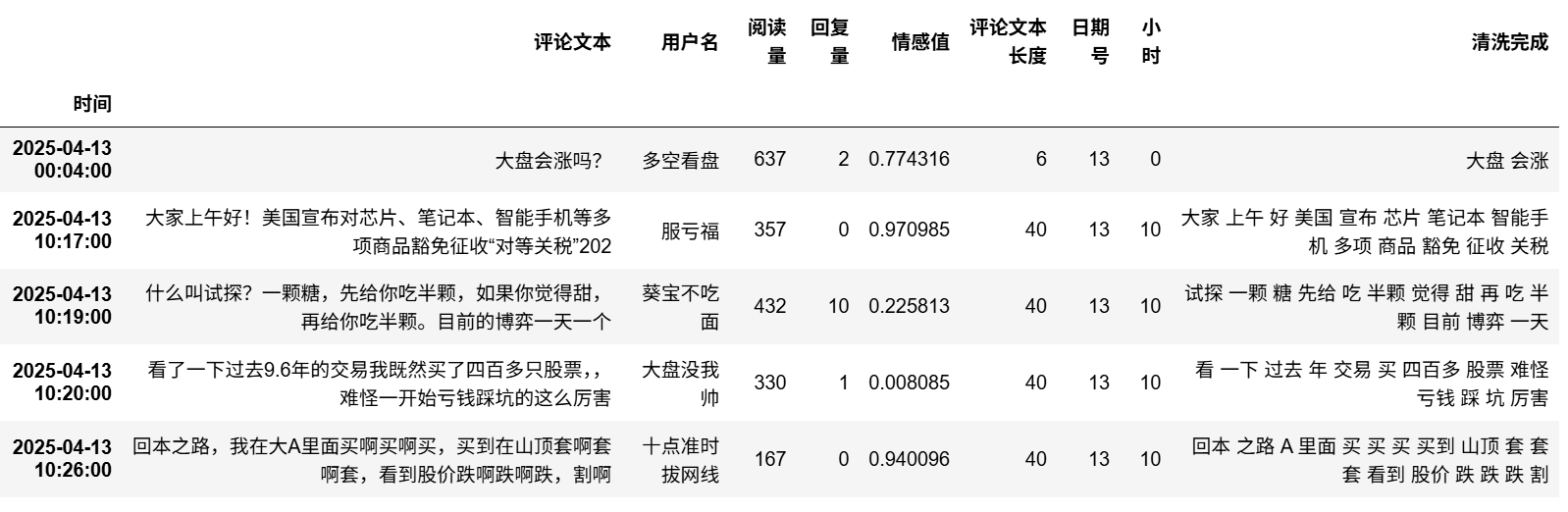
可以看到最后一类是分词处理完成的列,过滤掉的了很多语气词常用词等。
结巴分析
jieba库可以进行一定的权重抽取,查看最重要的前20的词汇:
import jieba.analyse
jieba.analyse.set_stop_words('停用词.txt')
jieba.analyse.set_stop_words
#合并一起
text = ''
for i in range(len(df['清洗完成'])):text += df['清洗完成'][i]+'\n'
jieba.analyse.extract_tags(text,topK=20,withWeight=True)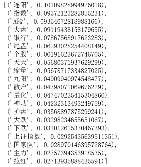
都是一些很长的股市评论讨论的词汇。
词袋分析
导入LDA模型的库
from sklearn.feature_extraction.text import  CountVectorizer,TfidfVectorizer
from sklearn.decomposition import LatentDirichletAllocation
from sklearn.preprocessing import MinMaxScalerimport gensim
import gensim.corpora as corpora
from gensim.models import CoherenceModel
from gensim.corpora.dictionary import Dictionary
词向量化
tf_vectorizer =CountVectorizer()
#tf_vectorizer = TfidfVectorizer(ngram_range=(2,2)) #2元词袋
X = tf_vectorizer.fit_transform(df['清洗完成'])
#print(tf_vectorizer.get_feature_names_out())
print(X.shape)feature_names = tf_vectorizer.get_feature_names_out()
tfidf_values = X.toarray()
print(feature_names.shape,tfidf_values.shape)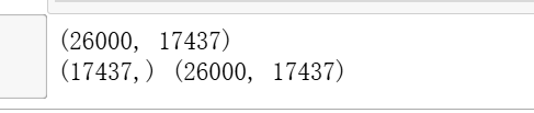
可以看到数据行数没变,2.6w行,列变成了17437列,都是词向量特征。
数值矩阵:
from scipy.sparse import coo_matrix
X_coo = coo_matrix(X)
df_tfidf = pd.DataFrame({'转换为数值向量的文本数据': list(zip(X_coo.row, X_coo.col)),'TF-IDF 值': X_coo.data
})
df_tfidf.head() 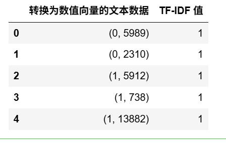
查看不同词汇和对应的 TF-IDF 值
# 从转换器中提取词汇和对应的 TF-IDF 值
data1 = {'word': tf_vectorizer.get_feature_names_out(),'frequency':np.count_nonzero(X.toarray(), axis=0),'weight': X.mean(axis=0).A.flatten(),}
df1 = pd.DataFrame(data1).sort_values(by="weight" ,ascending=False,ignore_index=True)
df1.head()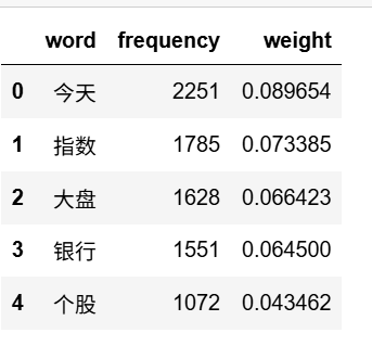
对前20的词汇进行可视化
df1=pd.DataFrame(data1).sort_values(by="weight" ,ascending=False,ignore_index=True)
plt.figure(figsize=(7,3),dpi=256)
sns.barplot(x=df1['word'][:20],y=df1['weight'][:20])
plt.xticks(rotation=70,fontsize=9)
plt.ylabel('TF-IDF')
plt.xlabel('')
#plt.title('前20个频率最高的词汇')
plt.show()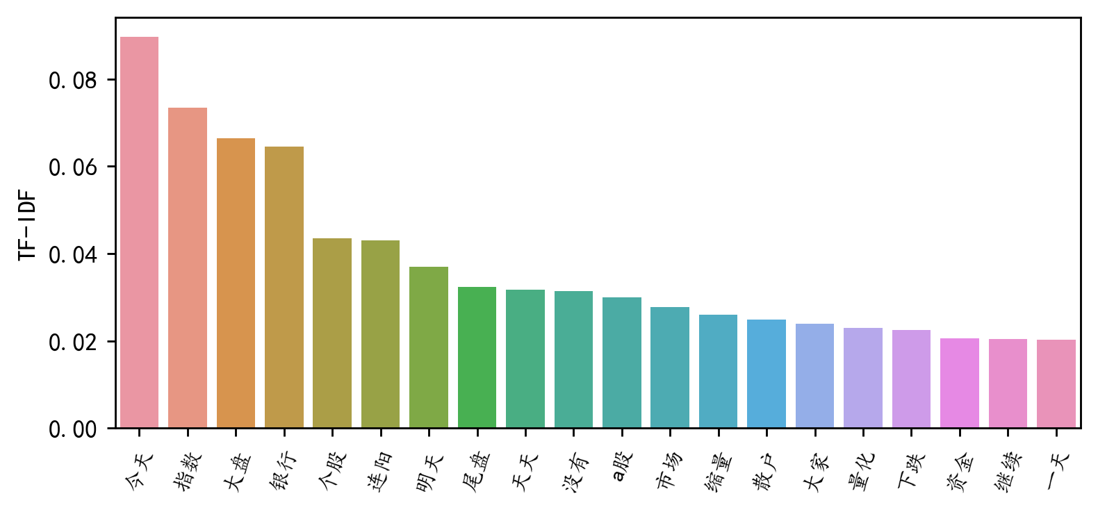
可以看到TF-IDF 值最高的前20 的词汇。
频率最高的前20的词汇
df2=pd.DataFrame(data1).sort_values(by="frequency" ,ascending=False,ignore_index=True)
plt.figure(figsize=(7,3),dpi=256)
sns.barplot(x=df2['word'][:20],y=df2['frequency'][:20])
plt.xticks(rotation=70,fontsize=9)
plt.ylabel('频率')
plt.xlabel('')
#plt.title('前20个频率最高的词汇')
plt.show()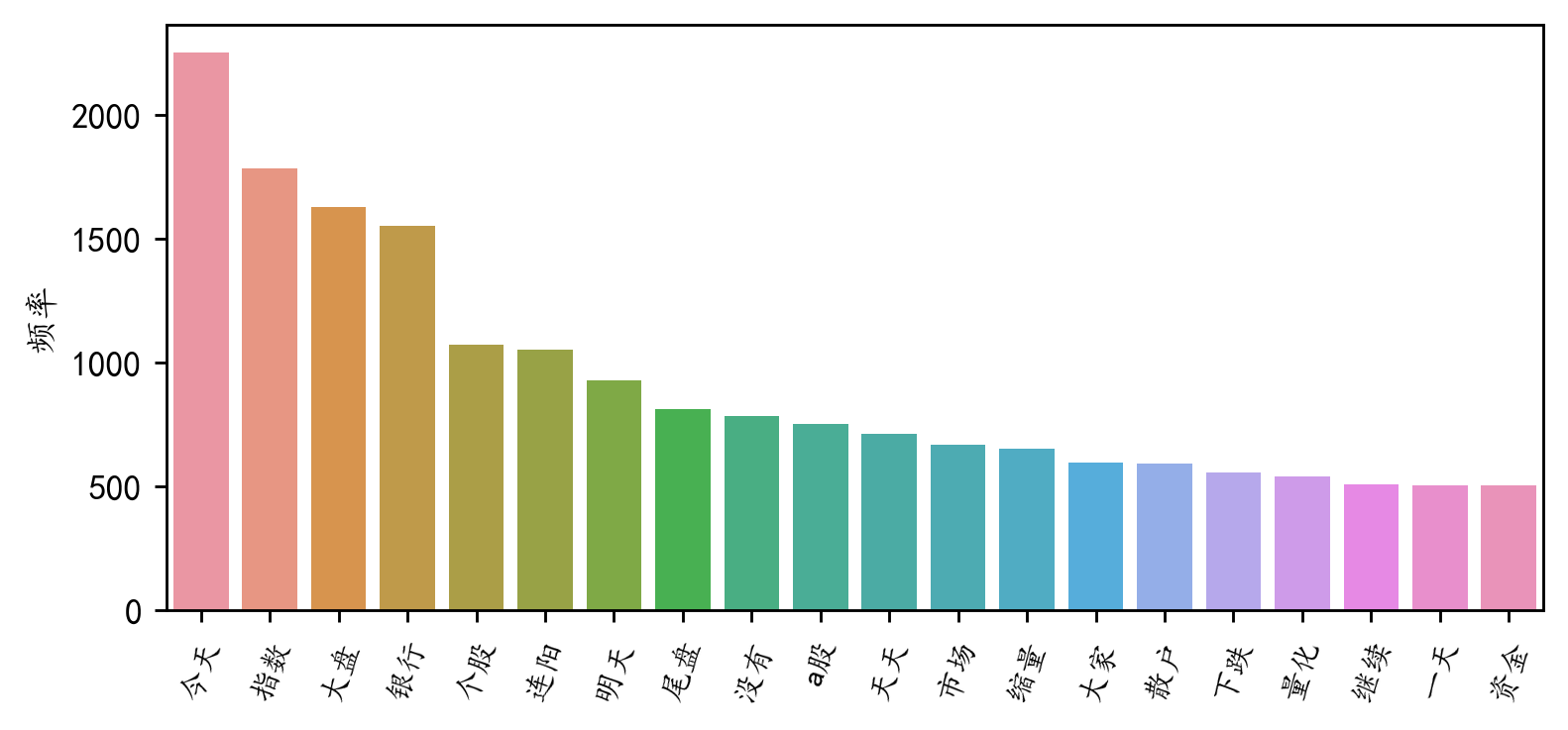
共线网络
将文本词汇构建为图结构的数据,节点就是词汇,如果在同一个评论里面,那么就可以构建一条边相连。边的数值大小取决于两个词同时出现的数值。
# 函数:提取高频词并构建共词矩阵
def build_cooccurrence_matrix(texts, top_n=200):# 分词并统计词频all_words = [word for text in texts for word in text.split()]most_common_words = [word for word, freq in Counter(all_words).most_common(top_n)]# 初始化共词矩阵cooccurrence_matrix = pd.DataFrame(np.zeros((top_n, top_n)), index=most_common_words, columns=most_common_words)# 构建共词矩阵for text in texts:words = text.split()# 只考虑高频词words = [word for word in words if word in most_common_words]for i, word1 in enumerate(words):for word2 in words[i + 1:]:if word2 in most_common_words:cooccurrence_matrix.at[word1, word2] += 1cooccurrence_matrix.at[word2, word1] += 1return cooccurrence_matrix
cooccurrence_matrix = build_cooccurrence_matrix(df['清洗完成'])
#cooccurrence_matrix.to_excel('共词矩阵.xlsx')
图结构的矩阵构建完成后,使用networkx进行可视化
import networkx as nx
# 函数:绘制共现网络
def plot_cooccurrence_network(cooccurrence_matrix):# 创建图G = nx.Graph()# 添加节点和边for word1 in cooccurrence_matrix.columns:for word2 in cooccurrence_matrix.index:weight = cooccurrence_matrix.at[word1, word2]if weight > 0:G.add_edge(word1, word2, weight=weight)# 设置节点大小degrees = dict(nx.degree(G))node_size = [v * 10 for v in degrees.values()]# 绘图plt.figure(figsize=(10, 10),dpi=128)nx.draw(G, with_labels=True, node_size=node_size, font_size=25, font_weight='bold', node_color='skyblue', edge_color='gray')plt.show()
plot_cooccurrence_network(cooccurrence_matrix.iloc[:20,:20])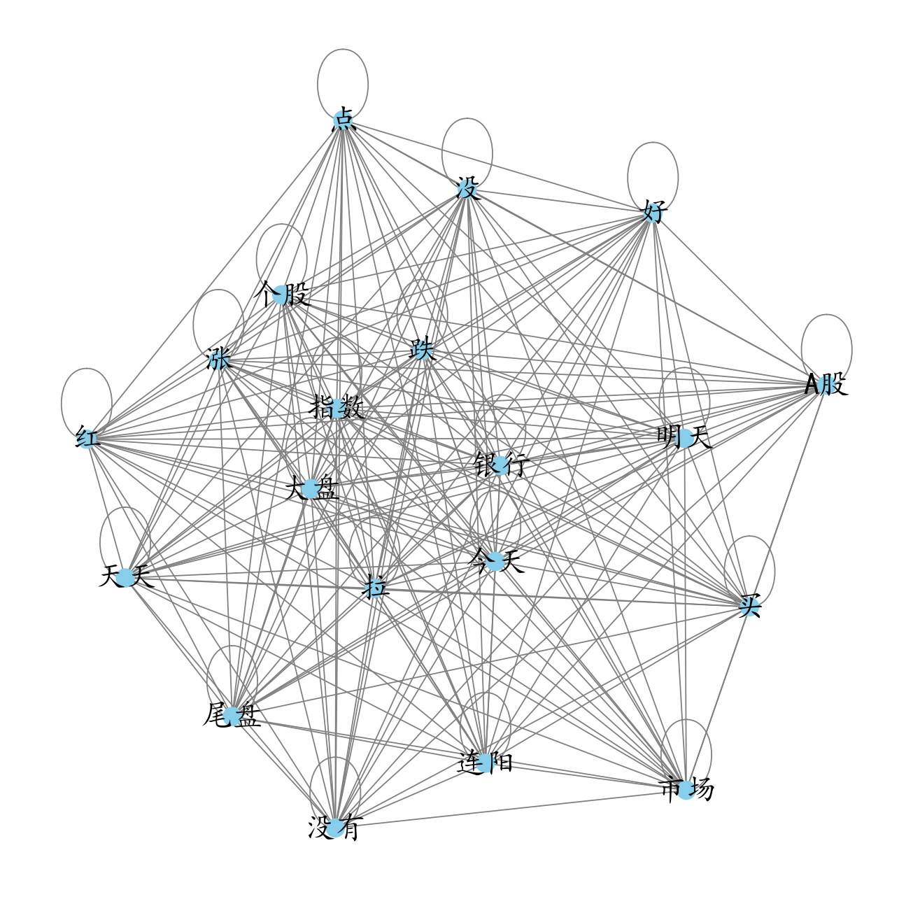
这个图没有弄得很精致,可以用ai改一下,颜色弄得好看一点,边的大小可以使用数值来表示,两个词汇数值越大越粗。
LDA建模
LDA是无监督的分类方法,对文本进行聚类,所以需要确定一下聚为几类比较好。
使用困惑度和一致性进行评价,定义函数:
def calculate_perplexity_coherence(X, tf_vectorizer, df_cutword, n_topics):"""Calculates perplexity and coherence for a given number of topics in LDA.:param X: Document-term matrix:param tf_vectorizer: TF vectorizer object:param df_cutword: Preprocessed text data for coherence calculation:param n_topics: Number of topics for LDA:return: A tuple of (perplexity, coherence)"""# Create and fit LDA modellda = LatentDirichletAllocation(n_components=n_topics, max_iter=50, learning_method='batch',learning_offset=100, random_state=0)lda.fit(X)# Calculate perplexityperplexity = lda.perplexity(X)# Prepare for coherence calculationwords = tf_vectorizer.get_feature_names_out()corpus = gensim.matutils.Sparse2Corpus(X, documents_columns=False)lda_topics = lda.components_ / lda.components_.sum(axis=1)[:, np.newaxis]top_words = [[words[i] for i in topic.argsort()[:-21:-1]] for topic in lda_topics]id2word = Dictionary([words])# Calculate coherencecoherence_model = CoherenceModel(topics=top_words, texts=df_cutword, corpus=corpus, dictionary=id2word, coherence='u_mass')coherence = coherence_model.get_coherence()return perplexity, coherencedef scale_data(values):values = np.array(values).reshape(-1, 1)scaler = MinMaxScaler(feature_range=(0, 1))scaled_values = scaler.fit_transform(values)return scaled_values.flatten().tolist()遍历1-20个类别,查看对应的困惑度和一致性。
perplexity=[] ; coherence=[]
for n in  range(1,20):print(f"{n}话题在拟合")p,n=calculate_perplexity_coherence(X, tf_vectorizer, df['清洗完成'], n_topics=n)perplexity.append(p)  ;  coherence.append(n)
可视化
coherence=scale_data(coherence)
def plot_perplexity_coherence(perplexity, coherence, topic_range):fig, axes = plt.subplots(1, 2, figsize=(12, 5), dpi=128)axes[0].plot(topic_range, perplexity, marker='o', color='b')axes[0].set_title('Perplexity vs Number of Topics')axes[0].set_xlabel('Number of Topics')axes[0].set_ylabel('Perplexity')axes[0].set_xticks(topic_range)  # 设置X轴刻度axes[1].plot(topic_range, coherence, marker='o', color='r')axes[1].set_title('Coherence vs Number of Topics')axes[1].set_xlabel('Number of Topics')axes[1].set_ylabel('Coherence')axes[1].set_xticks(topic_range)  # 设置X轴刻度plt.tight_layout()plt.show()
plot_perplexity_coherence(perplexity, coherence, range(1, 20))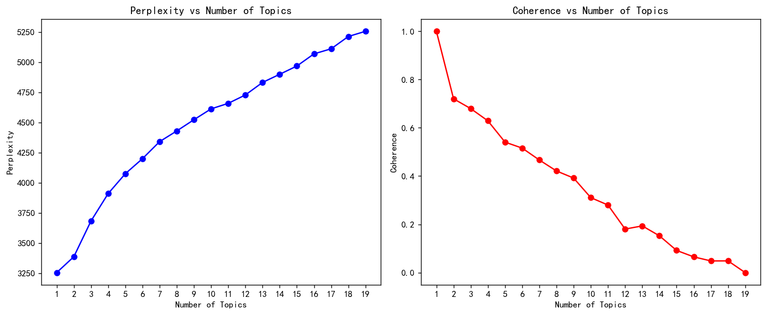
由于评论文本都比较短,所以这两个评价指标都是单调的。
本文就选择n为4比较好,困惑度低而且一致性还算比较高。
进行模型构建
n_topics = 4  #分为n类
lda = LatentDirichletAllocation(n_components=n_topics, max_iter=100,learning_method='batch',learning_offset=100,
#                                 doc_topic_prior=0.1,
#                                 topic_word_prior=0.01,random_state=0)
lda.fit(X)
# 计算困惑度
perplexity = lda.perplexity(X)
# 计算一致性
# 转换数据格式
words = tf_vectorizer.get_feature_names_out()
corpus = gensim.matutils.Sparse2Corpus(X, documents_columns=False)
#id2word = dict((v, k) for k, v in tf_vectorizer.vocabulary_.items())
perplexity
查看拟合的每个主题的对应词语和概率。
def print_top_words(model, feature_names, n_top_words):tword = [];tword2 = []tword3=[]for topic_idx, topic in enumerate(model.components_):print("Topic #%d:" % topic_idx)topic_w = [feature_names[i] for i in topic.argsort()[:-n_top_words - 1:-1]]topic_pro=[str(round(topic[i],3)) for i in topic.argsort()[:-n_top_words - 1:-1]] #(round(topic[i],3))tword.append(topic_w) tword2.append(topic_pro)print(" ".join(topic_w))print(" ".join(topic_pro))print(' ')word_pro=dict(zip(topic_w,topic_pro))tword3.append(word_pro)return tword3查看每个主题前20的词语
##输出每个主题对应词语和概率
n_top_words = 20
feature_names = tf_vectorizer.get_feature_names_out()
word_pro = print_top_words(lda, feature_names, n_top_words)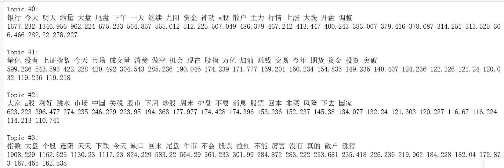
#输出每篇文章对应主题
topics=lda.transform(X)
topic=np.argmax(topics,axis=1)
df['topic']=topic
#df.to_excel("data_topic.xlsx",index=False)
print(topics.shape)
print(topics[0])
topic[0]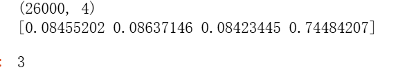
获取主题-词分布的结果,可以进行一下存储。
# 主题-词分布
topic_word_distributions = lda.components_
n_top_words = 100# 主题-词分布结果DataFrame
topic_word_df_list = []
for topic_idx, topic in enumerate(topic_word_distributions):top_features_ind = topic.argsort()[:-n_top_words - 1:-1]top_features = [feature_names[i] for i in top_features_ind]weights = topic[top_features_ind]df_word = pd.DataFrame({'Word': top_features, 'Weight': weights})df_word['topic'] = f'Topic {topic_idx + 1}'topic_word_df_list.append(df_word)topic_word_df = pd.concat(topic_word_df_list, ignore_index=True)
#topic_word_df.to_excel('主题-词分布结果.xlsx', index=False)doc_topic_distributions = lda.transform(X)
doc_topic_df = pd.DataFrame(doc_topic_distributions, columns=[f'Topic {i+1}' for i in range(n_topics)])
doc_topic_df['Dominant Topic'] = doc_topic_df.idxmax(axis=1)
#doc_topic_df.to_excel('文本-主题分布结果.xlsx', index=False)
词云图
对上面的LDA进行可视化,画出词云图,先定义一个随机生成颜色的函数
import random   #定义随机生成颜色函数
def randomcolor():colorArr = ['1','2','3','4','5','6','7','8','9','A','B','C','D','E','F']color ="#"+''.join([random.choice(colorArr) for i in range(6)])return color
[randomcolor() for i in range(3)]
from collections import Counter
from wordcloud import WordCloud
from matplotlib import colors
#from imageio import imread #形状设置
#mask = imread('爱心.png') def generate_wordcloud(tup):color_list=[randomcolor() for i in range(10)] #随机生成10个颜色wordcloud = WordCloud(background_color='white',font_path='simhei.ttf',#mask = mask, #形状设置max_words=20, max_font_size=50,random_state=42,colormap=colors.ListedColormap(color_list) #颜色).generate(str(tup))return wordcloud可视化
dis_cols = 2                  #一行几个
dis_rows = 3
dis_wordnum=20
plt.figure(figsize=(5 * dis_cols, 5 * dis_rows),dpi=128)
kind=n_topicsfor i in range(kind):ax=plt.subplot(dis_rows,dis_cols,i+1)most10 = [ (k,float(v)) for k,v in word_pro[i].items()][:dis_wordnum]  #高频词ax.imshow(generate_wordcloud(most10), interpolation="bilinear")ax.axis('off')ax.set_title("第{}类话题 前{}词汇".format(i,dis_wordnum), fontsize=30)
plt.tight_layout()
plt.show()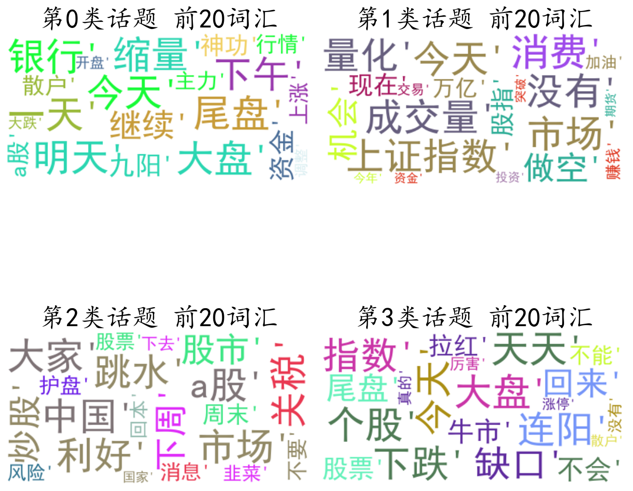
下面进行分析,分析报告如下:
LDA主题分析:股吧评论数据
根据LDA模型结果,股吧评论可划分为4个主题,每个主题的关键词及权重如下:
主题1:市场行情与主力资金动向
关键词:
银行(1677) | 大盘(565) | 资金(413) | 主力(379) | 上涨(314) | 大跌(306) | 调整(282)
主题分析:
- 聚焦A股整体走势,关注银行板块对大盘的影响
- 高频出现"缩量"、"尾盘"等交易时段技术分析词汇
- 包含"主力-散户"对立视角,反映投资者对资金博弈的关注
- 典型讨论:"今天银行股缩量调整,主力资金是否在尾盘撤离?"
主题2:量化交易与市场流动性
关键词:
量化(599) | 上证指数(543) | 成交量(285) | 做空(174) | 期货(121) | 突破(119) | 万亿(155)
主题分析:
- 关注量化交易对市场的影响,特别是成交量变化
- 出现"做空"、"股指期货"等衍生品相关术语
- "万亿"成交量成为重要观察指标
- 典型讨论:"今日成交量不足万亿,量化策略是否转向做空?"
主题3:政策消息与散户情绪
关键词:
A股(396) | 利好(274) | 关税(195) | 护盘(145) | 韭菜(121) | 风险(116) | 国家(111)
主题分析:
- 反映政策面消息(关税、护盘)对市场的影响
- 包含强烈情绪标签:"跳水"、"韭菜"、"回本"
- 体现散户对政策干预的期待
- 典型讨论:"关税利好出台为何A股反而跳水?国家队会护盘吗?"
主题4:技术分析与趋势判断
关键词:
指数(1908) | 连阳(1117) | 缺口(361) | 牛市(283) | 涨停(163) | 下跌(583) | 拉红(226)
主题分析:
- 强调技术指标分析(缺口、连阳、尾盘)
- 多空观点交织:"牛市"vs"下跌"
- 关注个股与大盘的背离现象
- 典型讨论:"指数三连阳但个股普跌,这个缺口必补!"
整体观察:
- 市场分层认知:机构视角(主题1/2)与散户视角(主题3)形成鲜明对比
- 情绪极化现象:同一主题内常同时出现"牛市"与"大跌"等对立词汇
- 政策敏感度:关税、护盘等关键词显示A股典型的"政策市"特征
- 技术分析主导:80%的关键词与K线形态、成交量等技术指标相关
写得这么好,这么有结构化当然是deepseek写的啦。
LDA有一个库可以进行可视化,在网页文件里面调整参数可以看到不同的主题和词频的情况
import pyLDAvis
import pyLDAvis.sklearn
pyLDAvis.enable_notebook()# 准备LDAvis数据
lda_vis = pyLDAvis.sklearn.prepare(lda, X, tf_vectorizer)# 保存为HTML文件
pyLDAvis.save_html(lda_vis, '股吧LDA.html')
运行完成后会在本地生成一个html文件
![]()
打开就可以看到LDA模型的美格主题的词汇,调整lambda参数的不同词汇的评论情况。这里就不展示。
总结
本文案例主要是构建一个lda模型,使用的是股吧的评论数据,对文本进行情感分析,主题分析,聚类分组聚合,最后得到的主题结果自己不会分析,可以让AI来分析,它们找文本词汇之间的关联性,并且进行解释是很强的。
本文是很常见的一个文本lda建模的全流程了。之前也写过几篇类似的文章,以后除非是有新的方法,否则应该不会再写lda类的模型了。本案例的数据获取上面数据介绍也有链接,也可以自己爬取。
创作不易,看官觉得写得还不错的话点个关注和赞吧,本人会持续更新python数据分析领域的代码文章~