VideoGrain:ICLR2025收录,无需训练,实现细粒度多层次视频编辑
1.简介
本文的核心动机是解决多粒度视频编辑(multi-grained video editing)中的关键挑战。多粒度视频编辑指的是在不同层次(类别级、实例级和部件级)上对视频内容进行精确编辑。尽管现有的扩散模型在视频生成和编辑方面取得了显著进展,但在多粒度编辑任务中仍面临两大主要问题:
-
语义错位(Semantic Misalignment):全局文本提示在所有帧上均匀应用时,导致文本特征无法精准集中在目标区域,降低了编辑的精确性。
-
特征耦合(Feature Coupling):扩散模型倾向于将不同实例视为同一类别的片段,导致特征混合,使得编辑时无法区分同一类别中的不同对象。
为了解决这些困难,作者提出了VideoGrain,一种Zero-shot方法,它通过调整时空(交叉和自)注意机制来实现对视频内容的细粒度控制。作者通过放大每个局部提示对相应的空间去纠缠区域的注意,同时最小化交叉注意中与不相关区域的交互,来增强文本到区域的控制。此外,作者还通过增加区域内的感知和减少区域间的干扰来改进特征分离。实验结果表明,该方法在实际场景中具有较好的检测性能。
项目地址:VideoGrain: Modulating Space-Time Attention for Multi-Grained Video Editing
github地址:GitHub - knightyxp/VideoGrain: [ICLR 2025] VideoGrain: This repo is the official implementation of "VideoGrain: Modulating Space-Time Attention for Multi-Grained Video Editing" 论文地址:[2502.17258] VideoGrain: Modulating Space-Time Attention for Multi-grained Video Editing
-
-
2.论文详解
随着扩散模型在视频生成和编辑领域的快速发展,现有的技术已经能够通过自然语言提示实现对视频内容的操控。然而,多粒度视频编辑——即在类别级(class-level)、实例级(instance-level)和部件级(part-level)上对视频进行修改——仍然是一个具有挑战性的问题。主要困难在于文本到区域控制的语义错位以及扩散模型内部的特征耦合,这些问题导致现有方法在编辑时无法精确区分同一类别中的不同实例,也无法在不干扰其他区域的情况下对特定区域进行修改。
为了克服这些挑战,作者提出了 VideoGrain,这是一种零样本方法,通过调节空间-时间注意力机制(包括交叉注意力和自注意力),实现对视频内容的细粒度控制。该方法的核心在于增强文本到区域的控制能力,同时保持不同区域之间的特征分离。具体来说,VideoGrain 通过放大每个局部提示对其对应空间区域的注意力,同时抑制对无关区域的注意力,从而解决语义错位问题。此外,通过增加区域内特征的关联并减少区域间特征的干扰,VideoGrain 有效避免了特征耦合,确保每个查询只关注其目标区域。
作者强调,VideoGrain 的目标是实现一种无需额外参数调整的零样本编辑方法,能够在现有基准和真实视频上实现多粒度视频编辑。这一方法的提出不仅为视频编辑领域带来了新的可能性,也为未来的研究提供了一个新的方向,即如何在不依赖大量训练数据的情况下,实现对视频内容的精确控制和编辑。
-
动机
为了研究为什么以前的方法在实例级视频编辑中失败(见图2),作者开始对扩散模型中的自注意和交叉注意特征进行基本分析。
如图3(B)所示,作者在DDIM反转期间将K均值聚类应用于每帧自注意特征。虽然聚类捕获了清晰的语义布局,但它无法区分不同的实例(例如,“左人”和“右人”)。增加聚类的数量会导致在部分级别进行更精细的分割,但并不能解决这个问题,这表明跨实例的特征同质性限制了扩散模型在多粒度视频编辑中的有效性。
接下来,作者尝试使用SDedit将同一类的两个人编辑到不同的实例中。然而,图3(d)显示“Iron Man”和“Spiderman”的权重在左边的人上重叠,而“blossom”的权重泄漏到右边的人上,导致(c)中的编辑失败。因此,对于有效的多粒度编辑,作者提出了以下问题:能否调节注意力以确保每个局部编辑的注意力权重准确地分布在预期区域中?
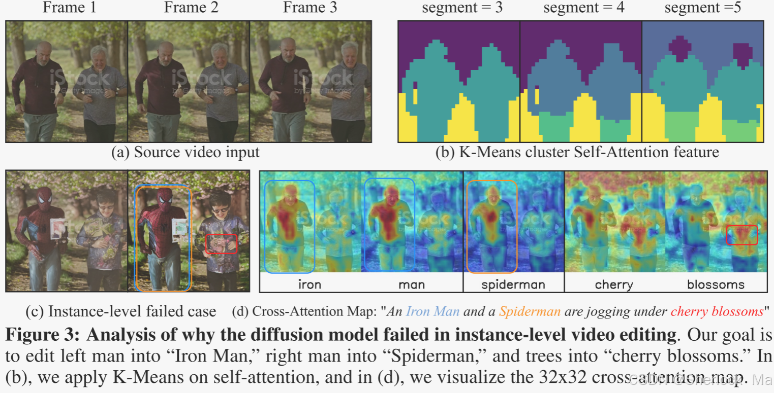
为了回答这个问题,作者提出了两个关键设计的VideoGrain:(1)调整交叉注意,诱导文本特征聚集在相应的空间分离区域,从而实现文本到区域的控制。(2)跨时空轴调节自我注意力,以增强区域内聚焦并减少区域间干扰,避免扩散模型内的特征耦合。
-
问题定义
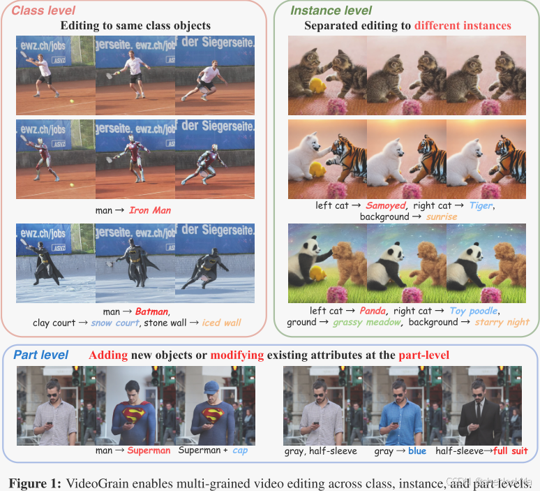
这项工作的目的是根据给定的提示在多个区域执行多粒度视频编辑。这涉及三个层次:
- (1)类级编辑:编辑同一类内的对象。(e.g.,将两个人改变为“蜘蛛侠”,其中两个人都属于人类类,如图2第二列所示)
- (2)实例级编辑:将每个单独的实例编辑为不同的对象。(e.g.,编辑左人为“蜘蛛侠”,右人为“北极熊”,如图2第三列所示)。
- (3)部件级编辑:将零件级编辑应用于各个实例的特定图元。(e.g.,当编辑图2第四列中的“北极熊”时,将“太阳镜“添加到合适的人)。
作者的目标是通过调节每个区域的位置及其文本提示来改善视频编辑中的多粒度控制。
-
整体框架
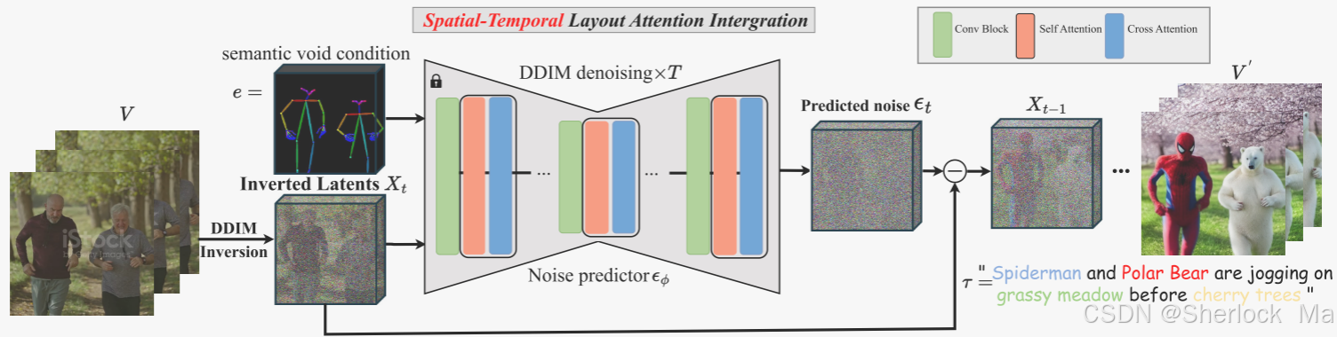
作者所提出的zero-shot多粒度视频编辑流水线在图4顶部中给出。
最初,为了保持高保真度,作者在干净的潜在信息上执行DDIM反演,以得到噪声潜在信息
。在反演过程之后,作者对自注意特征进行聚类以获得如图3(B)中的语义布局。由于自注意力特征不能单独区分个体实例,因此作者进一步采用SAM-Track来分割每个实例。最后,在去噪过程中,作者引入了ST-Layout Attn来调节交叉注意力和自注意力,以进行文本到区域的控制,并保持区域之间的特征分离。
与所有帧的一个全局文本提示控件不同,VideoGrain允许在去噪过程中指定成对的实例级或部件级提示及其位置。该方法也适用于ControlNet的条件e,它可以是深度或姿态图来提供结构条件。
-
时空布局引导注意
根据之前的观察,交叉注意力权重分布与编辑结果一致。与此同时,自注意力对于生成时间一致的视频也至关重要。然而,一个区域中的像素可能会关注外部或相似区域,这对多粒度视频编辑构成了障碍。因此,需要调节自我注意和交叉注意,使每个像素或局部提示只关注正确的区域。
为了实现这一目标,作者通过统一的增加积极和减少消极的方式来调节交叉注意和自注意机制。具体地,对于Query特征的第i帧,作者以如下方法调整Query-Key QK查询条件映射:
,其中:
指示帧i处的Query-Key对的条件映射,是操纵是增加还是减少特定对的注意力分数。
是正则化项。Ri 用于调节交叉注意力(cross-attention)和自注意力(self-attention)的权重分布。它的作用是控制哪些查询-键对(query-key pairs)的注意力权重需要增加(正对),哪些需要减少(负对)。
控制跨时间步长的调制强度,从而允许形状和外观细节的逐渐细化。
-
调节交叉注意力以进行文本到区域控制
在交叉注意层中,文本特征作为关键字和值,与来自视频潜特征的查询特征进行交互。由于每个实例的外观和位置与交叉注意权重分布密切相关,因此作者的目标是鼓励每个实例的文本特征聚集在相应的位置。
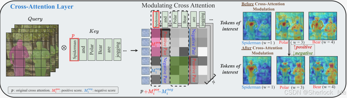
如图所示,给定布局条件()。例如,对于
= Spiderman,在Query-Key交叉注意力映射中,我们可以手动指定查询特征中对应于m1的部分为正,而所有其余部分都指定为负。因此,对于每个帧i,可以将交叉关注层中的调制值设置为:
,其中
- x和y是查询和键索引,
是交叉关注层中的查询-键条件映射。通过最初将每个区域的掩码
广播到其对应的文本key embedding
来正则化此条件映射,从而产生条件映射
。
上述公式定义了交叉注意力中正对(positive pair)和负对(negative pair)的注意力权重调节值,目的是增强文本提示(text prompt)与目标区域之间的关联,同时抑制对无关区域的注意力。
-
增强正对的注意力:通过增加正对的注意力权重,使得文本提示能够更精准地集中在目标区域。
的含义是:通过将每个位置的注意力权重与最大值的差距作为调节值,增强正对的注意力权重。这样可以使得目标区域的注意力权重更高,从而更精准地影响目标区域。
-
抑制负对的注意力:通过减少负对的注意力权重,避免文本特征对无关区域的影响。
的含义是:通过将每个位置的注意力权重与最小值的差距作为调节值,减少负对的注意力权重。这样可以抑制文本特征对无关区域的影响。
-
-
调节自我注意力以保持特征分离
为了使T2I模型适用于T2V编辑,作者将完整的视频视为“更大的画面”,用时空自我注意力取代空间注意力,同时保留预训练的权重。这增强了跨框架的交互,并提供了更广泛的视觉环境。然而,原生的自注意力可能会导致区域关注不相关或相似的区域(例如,图4底部,在调制查询p参加两人)之前,这导致混合纹理。为了解决这个问题,我们需要加强同一区域内的积极关注,限制不同区域之间的负面互动。
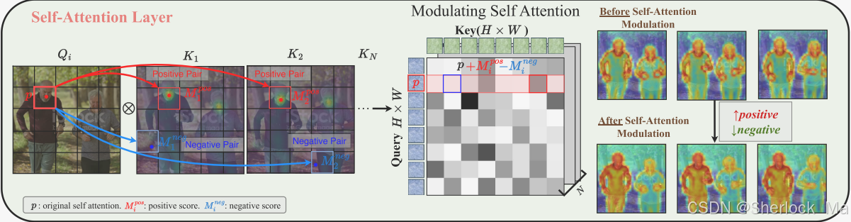
如图所示,最大跨帧扩散特征指示同一区域内的标记中的最强响应。注意,DIFT使用它来匹配不同的图像,而作者专注于生成过程中的跨帧对应和区域内注意调制。然而,负区域间对应对于解耦特征混合同样至关重要。除了DIFT之外,作者发现最小跨帧扩散特征相似性有效地捕获了不同区域的令牌之间的关系。因此,作者将时空正/负值定义为:
,其中
- 对于帧索引i和j,当令牌属于跨帧的不同实例时,该值为零。
-
Qi 是第 i 帧的查询特征。
-
[K1,…,Kn] 是所有帧的键特征。
该公式通过定义正对(positive pair)和负对(negative pair)的调节值,来增强区域内特征的关联并减少区域间特征的干扰。
-
的计算方式是:最大注意力权重减去原始注意力权重,表示每个查询与键之间的正对调节值。通过
-
的计算方式是:原始注意力权重减去最小注意力权重,表示每个查询与键之间的负对调节值。通过
如图右侧部分所示,在应用作者的自注意力调整之后,来自左边男人的鼻子的查询特征(例如,p)只注意左边的实例,避免分心到右边的实例。这表明我们的自我注意调制打破了扩散模型的类级特征对应,确保了实例级的特征分离。
-
实验
作者在视频上评估VideoGrain,包括类级、实例级和部件级编辑。
图5展示了处理动物的能力,例如将“狼”转化为“猪”(图5,左上)。对于实例级编辑,我们可以单独修改车辆(例如,将“SUV”变换为“消防车”,将“货车”变换为“校车”)。VideoGrain擅长在复杂、闭塞的场景中编辑多个实例,比如“蜘蛛侠和神奇女侠打羽毛球”(图5,中左)。以前的方法经常在这种非刚性运动中发生错误。此外,作者的方法能够进行多区域编辑,其中前景和背景都被编辑,其中背景变为“森林中湖泊上的苔藓石桥”(图5,中右)。由于精确的注意力权重分布,我们可以无缝地交换身份,例如在慢跑场景中,“钢铁侠”和“蜘蛛侠”交换身份(图5,左下)。对于部分级别的编辑,VideoGrain擅长将角色调整为穿着超人套装,同时保持太阳镜完好无损(图5,右下)。总体而言,对于多粒度编辑,作者的VideoGrain表现出出色的性能。
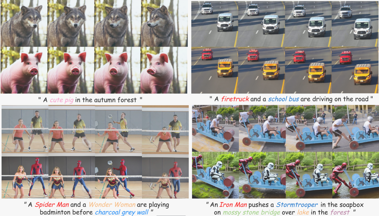
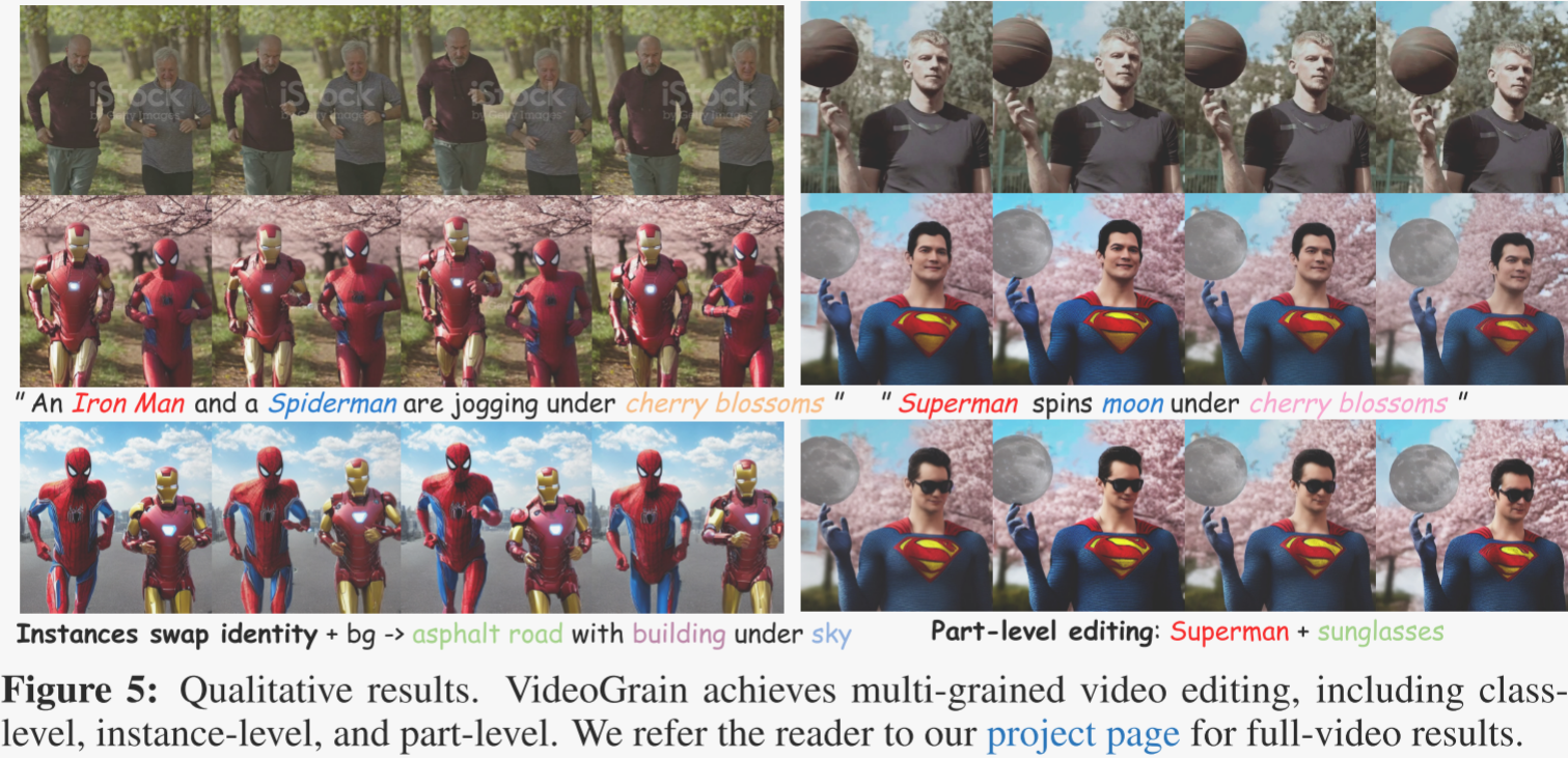
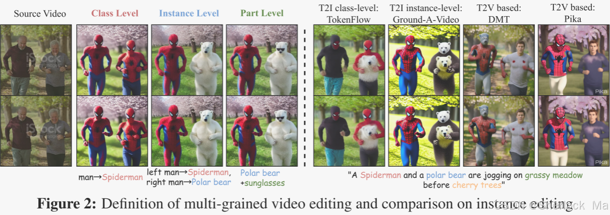
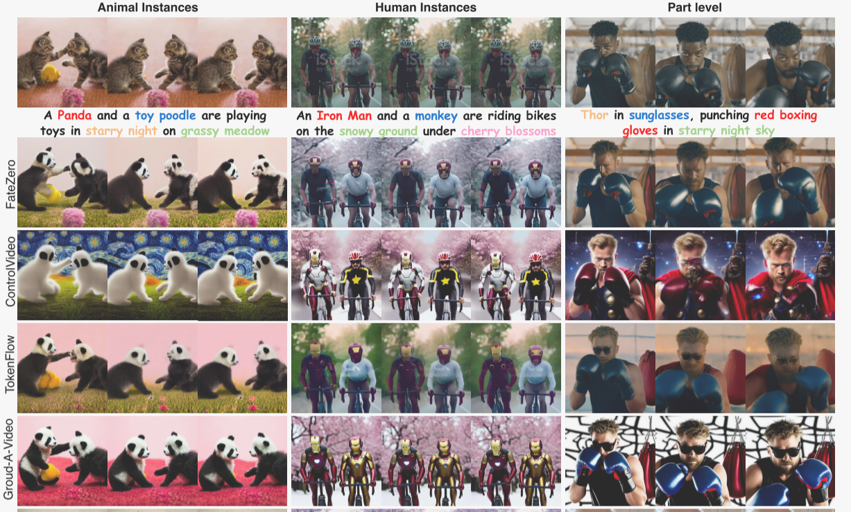
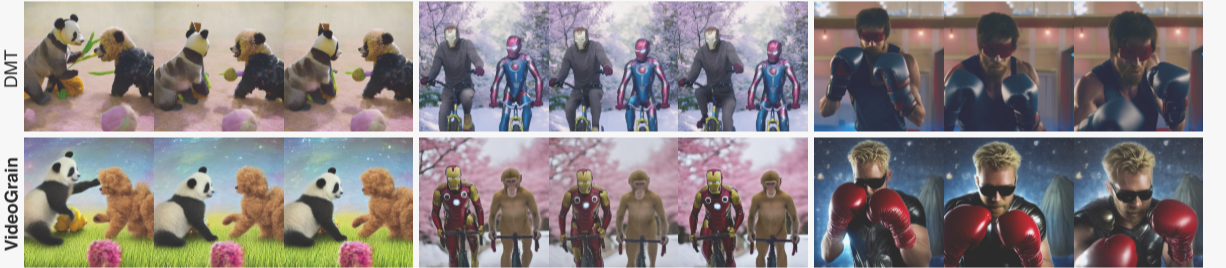
图6显示了VideoGrain和基线方法之间的比较,包括基于T2I和基于T2V的方法,用于实例级和部件级编辑。为了公平起见,所有基于T2I的方法都使用ControlNet条件。
(1)动物实例:在左列中,基于T2I的方法,如FateZero,ControlVideo和TokenFlow,由于扩散模型中的同类特征耦合,无法执行单独的将两只猫编辑为熊猫。DMT即使有视频生成先验,仍然混合了熊猫和玩具贵宾犬的特征。相比之下,VideoGrain成功地将一只编辑成熊猫,另一只编辑成玩具贵宾犬。
(2)人类实例:在中间的一列中,基线在同类实例发生冲突,DMT和Groud-A-Video也未能遵循用户意图,错误地编辑了左,右实例。然而,VideoGrain正确地将右边的人变成了猴子,打破了同类限制。
(3)部件级编辑:在第三列中,VideoGrain管理部件级编辑,例如太阳镜和拳击手套。ControlVideo编辑手套,但与太阳镜发生运动一致性冲突。TokenFlow和DMT编辑太阳镜,但无法修改手套或背景。相比之下,VideoGrain实现了实例级和部件级编辑,显著优于以前的方法。
-
-
3.代码详解
环境配置
安装虚拟环境,需要Python=3.10,CUDA=12.1
然后分别安装所需包:
# Step 2: Install PyTorch, CUDA and Xformers
conda install pytorch==2.3.1 torchvision==0.18.1 torchaudio==2.3.1 pytorch-cuda=12.1 -c pytorch -c nvidia
pip install --pre -U xformers==0.0.27
# Step 3: Install additional dependencies with pip
pip install -r requirements.txt
下载所需权重,也可以参考ckpt/download.sh手动下载
## download sd 1.5, controlnet depth/pose v10/v11
bash download_all.sh
下载其他权重,并将其解压到./annotator/ckpts
- 谷歌:https://drive.google.com/file/d/1qOsmWshnFMMr8x1HteaTViTSQLh_4rle/view?usp=drive_link
- 百度:百度网盘 请输入提取码
下载所需数据,也可以手动下载
gdown https://drive.google.com/file/d/1dzdvLnXWeMFR3CE2Ew0Bs06vyFSvnGXA/view?usp=drive_link
tar -zxvf videograin_data.tar.gz
然后即可开始推理:
bash test.sh
#or
CUDA_VISIBLE_DEVICES=0 accelerate launch test.py --config config/part_level/adding_new_object/run_two_man/running_spider_polar_sunglass.yaml
结果会被保存在result文件夹下
result
├── run_two_man
│   ├── control                         # control conditon
│   ├── infer_samples
│           ├── input                   # 输入视频(帧)的文件夹
│           ├── masked_video.mp4        # 检查编辑区域是否被准确覆盖
│   ├── sample
│           ├── step_0                  # 结果(帧)
│           ├── step_0.mp4              # 结果(视频)
│           ├── source_video.mp4        # 输入视频
│           ├── visualization_denoise   # cross attention 权重
│           ├── sd_study                # 聚类 inversion 特征
-
整体流程
代码首先运行run()函数,然后进入test()函数运行,test()函数刚开始的初始化、加载权重不多介绍了。
这段代码的主要功能是处理数据集并生成样本。具体步骤如下:
- 使用 tokenizer 将数据集中的提示文本转换为模型输入格式。
- 创建 ImageSequenceDataset 数据集实例,传入配置和处理后的提示文本。
- 构建 DataLoader,用于批量加载数据。
- 保存训练样本到指定路径。
prompt_ids = tokenizer(     # 处理提示词 [batch_size, tokenizer.model_max_length]=[1,77]
    dataset_config["prompt"],
    truncation=True,
    padding="max_length",
    max_length=tokenizer.model_max_length,      # 77
    return_tensors="pt",
).input_ids

video_dataset = ImageSequenceDataset(**dataset_config, prompt_ids=prompt_ids)   # 创建 ImageSequenceDataset 数据集实例,传入配置和处理后的提示文本。

train_dataloader = torch.utils.data.DataLoader(     # 构建 DataLoader,用于批量加载数据。
    video_dataset,
    batch_size=batch_size,
    shuffle=True,
    num_workers=4,
    collate_fn=collate_fn,
)

train_sample_save_path = os.path.join(logdir, "infer_samples")      # 保存训练样本到指定路径
log_infer_samples(save_path=train_sample_save_path, infer_dataloader=train_dataloader)
这段代码定义了一个生成器函数 make_data_yielder,用于无限循环地从数据加载器中获取批次数据,并确保所有进程同步。这段代码定义了一个生成器函数 make_data_yielder,用于无限循环地从数据加载器中获取批次数据,并确保所有进程同步。
def make_data_yielder(dataloader):      # 接收一个数据加载器作为参数。
    while True:
        for batch in dataloader:
            yield batch     # 通过 yield 返回批次数据。
        accelerator.wait_for_everyone()

train_data_yielder = make_data_yielder(train_dataloader)    # 定义了一个生成器函数 make_data_yielder,用于无限循环地从数据加载器中获取批次数据


batch = next(train_data_yielder)    # 创建生成器实例 train_data_yielder 并从中获取一个批次数据。
生成骨架图
control = []
for i in images:
    img = i.cpu().numpy()
    i = img.astype(np.uint8)

    if xx:
        ......
    elif control_type == 'dwpose':      # 用DWposeDetector来检测图像中的人体姿态,并生成相应的控制图。
        detected_map = apply_control(i, hand=control_config['hand'], face=control_config['face'])
    ......
    control.append(HWC3(detected_map))      # 该函数 HWC3 用于将输入图像转换为 HWC 格式(高度、宽度、通道),并确保输出图像的通道数为 3。
默认调用DWpose进行姿态生成,其位于annotator/dwpose下
这段代码定义了 DWposeDetector 类的 __call__ 方法,用于处理输入图像并返回绘制了姿态信息的图像。主要步骤如下:
- 复制输入图像并获取其尺寸。
- 使用 torch.no_grad() 禁用梯度计算,调用 self.pose_estimation(oriImg) 进行姿态估计,得到候选点和子集。
- 对候选点进行归一化处理,并根据阈值筛选可见的关键点。
- 将候选点分为身体、脚、脸和手部分。
- 构建包含身体、手和脸的姿态字典。
- 调用 draw_pose 函数绘制姿态图。
这部分使用现有模型进行处理,且不是重点,故不多介绍。
class DWposeDetector:
    def __init__(self):

        self.pose_estimation = Wholebody()

    def __call__(self, oriImg,hand=False, face=False):
        oriImg = oriImg.copy()
        H, W, C = oriImg.shape
        with torch.no_grad():
            candidate, subset = self.pose_estimation(oriImg)    # 用 self.pose_estimation(oriImg) 进行姿态估计,得到候选点和子集。
            nums, keys, locs = candidate.shape
            candidate[..., 0] /= float(W)       # 对候选点进行归一化处理
            candidate[..., 1] /= float(H)
            body = candidate[:,:18].copy()
            body = body.reshape(nums*18, locs)
            score = subset[:,:18]
            for i in range(len(score)):         # 并根据阈值筛选可见的关键点。
                for j in range(len(score[i])):
                    if score[i][j] > 0.3:
                        score[i][j] = int(18*i+j)
                    else:
                        score[i][j] = -1

            un_visible = subset<0.3
            candidate[un_visible] = -1
            # 将候选点分为身体、脚、脸和手部分。
            foot = candidate[:,18:24]

            faces = candidate[:,24:92]

            hands = candidate[:,92:113]
            hands = np.vstack([hands, candidate[:,113:]])

            bodies = dict(candidate=body, subset=score)
            pose = dict(bodies=bodies, hands=hands, faces=faces)

            return draw_pose(pose, H, W, draw_body=True, draw_hand=hand, draw_face=face)    # 调用 draw_pose 函数绘制姿态图。
这段代码的主要功能是处理和保存控制图:将控制图数据堆叠并归一化,然后转换为PyTorch张量并调整维度,最后将处理后的控制图添加到批次数据中。
control = np.stack(control)
control = np.array(control).astype(np.float32) / 255.0      # 归一化
control = torch.from_numpy(control).to(accelerator.device)
control = control.unsqueeze(0) #[f h w c] -> [b f h w c ]
control = rearrange(control, "b f h w c -> b c f h w")
control = control.to(weight_dtype)
batch['control'] = control      # 处理后的控制图添加到批次数据中

control_save = control.cpu().float()

print("save control")

control_save_dir = os.path.join(logdir, "control")

save_tensor_images_and_video(control_save, control_save_dir)
计算光流和采样轨迹
## 计算光流和采样轨迹
trajectories = sample_trajectories_new(os.path.join(logdir, "source_video.mp4"),accelerator.device,height,width)
该函数 sample_trajectories_new 用于从视频中采样轨迹。主要步骤如下:
- 读取视频帧并进行预处理。
- 使用 Raft-Large 模型估计光流。
- 根据不同分辨率生成轨迹,并处理冲突点。
- 创建轨迹序列及其掩码,返回结果。
#=============== raft-large estimate forward optical flow============#
model = raft_large(weights=Raft_Large_Weights.DEFAULT, progress=False).to(device)       # Raft-Large 模型,用于估计光流
model = model.eval()
finished_trajectories = []

current_frames, next_frames = preprocess(frames[clips[:-1]], frames[clips[1:]], transforms, height,width)       # 对两批数据(当前帧和下一帧)进行光流估计
list_of_flows = model(current_frames.to(device), next_frames.to(device))    # 使用预训练的Raft-Large模型估计当前帧和下一帧之间的光流。
predicted_flows = list_of_flows[-1]     # 获取最终的光流预测结果。
#=============== raft-large estimate forward optical flow============#
光流估计并不是本文的重点,因此不多介绍,必要的注释已在下面写出
for resolution in resolutions:
    print("="*30)
    # print(resolution)
    # print('window_sizes[resolution]',window_sizes[resolution])
    trajectories = {}
    height_scale_factor = resolution[0] / height
    width_scale_factor = resolution[1] / width
    predicted_flow_resolu = torch.round(max(resolution[0], resolution[1])*torch.nn.functional.interpolate(predicted_flows, scale_factor=(height_scale_factor, width_scale_factor)))     # 根据光流预测结果生成缩放后的光流图

    T = predicted_flow_resolu.shape[0]+1
    H = predicted_flow_resolu.shape[2]
    W = predicted_flow_resolu.shape[3]

    is_activated = torch.zeros([T, H, W], dtype=torch.bool)     # 初始化激活状态矩阵 is_activated

    for t in range(T-1):        # 遍历视频帧的每个像素点,根据光流预测结果生成轨迹。
        flow = predicted_flow_resolu[t]
        for h in range(H):
            for w in range(W):

                if not is_activated[t, h, w]:
                    is_activated[t, h, w] = True
                    # this point has not been traversed, start new trajectory
                    x = h + int(flow[1, h, w])
                    y = w + int(flow[0, h, w])
                    if x >= 0 and x < H and y >= 0 and y < W:
                        # trajectories.append([(t, h, w), (t+1, x, y)])
                        trajectories[(t, h, w)]= (t+1, x, y)
    # 处理轨迹中的冲突点,确保每个点只属于一条轨迹。
    conflict_points = keys_with_same_value(trajectories)    # 使用 keys_with_same_value 函数找出所有具有相同值的键,即冲突点。
    for k in conflict_points:
        index_to_pop = random.randint(0, len(conflict_points[k]) - 1)       # 对每个冲突点集合,随机移除一个点。
        conflict_points[k].pop(index_to_pop)
        for point in conflict_points[k]:
            if point[0] != T-1:
                trajectories[point]= (-1, -1, -1) # stupid padding with (-1, -1, -1)    将剩余的冲突点标记为无效轨迹,用 (-1, -1, -1) 填充。

    active_traj = []
    all_traj = []
    for t in range(T):
        pixel_set = {(t, x//H, x%H):0 for x in range(H*W)}
        new_active_traj = []
        for traj in active_traj:    # 遍历当前活动轨迹active_traj,检查每个轨迹的最后一个点是否在trajectories中。
            if traj[-1] in trajectories:    # 如果存在,则将该轨迹扩展,并标记新的点。
                v = trajectories[traj[-1]]
                new_active_traj.append(traj + [v])
                pixel_set[v] = 1
            else:       # 否则,将该轨迹添加到all_traj中
                all_traj.append(traj)
        active_traj = new_active_traj
        active_traj+=[[pixel] for pixel in pixel_set if pixel_set[pixel] == 0]
    all_traj += active_traj

    useful_traj = [i for i in all_traj if len(i)>1]     # 筛选出长度大于1的轨迹,存入 useful_traj。
    for idx in range(len(useful_traj)):         # 遍历 useful_traj,如果轨迹的最后一个点是无效点,则将其移除。
        if useful_traj[idx][-1] == (-1, -1, -1):
            useful_traj[idx] = useful_traj[idx][:-1]
    print("how many points in all trajectories for resolution{}?".format(resolution), sum([len(i) for i in useful_traj]))
    print("how many points in the video for resolution{}?".format(resolution), T*H*W)

    # validate if there are no duplicates in the trajectories
    trajs = []
    for traj in useful_traj:
        trajs = trajs + traj
    assert len(find_duplicates(trajs)) == 0, "There should not be duplicates in the useful trajectories."

    # check if non-appearing points + appearing points = all the points in the video
    all_points = set([(t, x, y) for t in range(T) for x in range(H) for y in range(W)])
    left_points = all_points- set(trajs)
    print("How many points not in the trajectories for resolution{}?".format(resolution), len(left_points))
    for p in list(left_points):
        useful_traj.append([p])
    print("how many points in all trajectories for resolution{} after pending?".format(resolution), sum([len(i) for i in useful_traj]))


    longest_length = max([len(i) for i in useful_traj])
    sequence_length = (window_sizes[resolution]*2+1)**2 + longest_length - 1

    seqs = []
    masks = []

    # create a dictionary to facilitate checking the trajectories to which each point belongs.
    point_to_traj = {}      # 创建一个字典 point_to_traj,用于快速查找每个点所属的轨迹。
    for traj in useful_traj:
        for p in traj:
            point_to_traj[p] = traj

    for t in range(T):      # 遍历所有时间帧、高度和宽度的像素点,获取每个点的邻居。
        for x in range(H):
            for y in range(W):
                neighbours = neighbors_index((t,x,y), window_sizes[resolution], H, W)
                sequence = [(t,x,y)]+neighbours + [(0,0,0) for i in range((window_sizes[resolution]*2+1)**2-1-len(neighbours))]
                sequence_mask = torch.zeros(sequence_length, dtype=torch.bool)
                sequence_mask[:len(neighbours)+1] = True

                traj = point_to_traj[(t,x,y)].copy()    # 获取当前点的完整轨迹
                traj.remove((t,x,y))
                sequence = sequence + traj + [(0,0,0) for k in range(longest_length-1-len(traj))]   # 将其添加到序列中
                sequence_mask[(window_sizes[resolution]*2+1)**2: (window_sizes[resolution]*2+1)**2 + len(traj)] = True  # 更新掩码

                seqs.append(sequence)
                masks.append(sequence_mask)

    seqs = torch.tensor(seqs)
    masks = torch.stack(masks)
    res["traj{}".format(resolution[0])] = seqs
    res["mask{}".format(resolution[0])] = masks
return res
预计算潜在变量
# 预计算这段视频的潜变量,使训练和测试中的初始潜变量保持一致

latents, attn_inversion_dict = pipeline.prepare_latents_ddim_inverted(
    image=rearrange(batch["images"].to(dtype=weight_dtype), "b c f h w -> (b f) c h w"),
    batch_size = 1,
    source_prompt = dataset_config.prompt,
    do_classifier_free_guidance=True,
    control=batch['control'], controlnet_conditioning_scale=control_config['controlnet_conditioning_scale'],
    use_pnp=editing_config['use_pnp'],
    cluster_inversion_feature=editing_config.get('cluster_inversion_feature', False),
    trajs=trajectories,
    old_qk=editing_config["old_qk"],
    flatten_res=editing_config['flatten_res']
)
该函数 prepare_latents_ddim_inverted 主要用于准备潜在变量(latents)以进行DDIM逆向推理。具体步骤如下:
- 初始化设备、时间步和一些保存特征的列表。
- 对输入的 prompt 进行编码,生成提示嵌入。
- 准备视频潜在变量。
- 使用进度条循环遍历逆向时间步,计算噪声预测并更新潜在变量。
- 如果使用 PnP,保存特定层的特征。
- 如果启用聚类反转特征,计算自注意力和交叉注意力的平均值,并进行 PCA 和聚类分析。
- 将聚类结果与名词关联,并保存相关掩码图像。
初始化如下:
# ddim inverse
num_inverse_steps = 50
self.inverse_scheduler.set_timesteps(num_inverse_steps, device=device)
inverse_timesteps, num_inverse_steps = self.get_inverse_timesteps(num_inverse_steps, 1, device)     # 获取逆向时间步和逆向步数。
num_warmup_steps = len(inverse_timesteps) - num_inverse_steps * self.inverse_scheduler.order        # 根据逆向时间步和逆向步数计算预热步骤数。

#============ddim inversion==========*
prompt_embeds = self._encode_prompt(    # 对prompt进行编码,生成提示嵌入prompt_embeds。
    source_prompt,
    device=device,
    num_images_per_prompt=1,
    do_classifier_free_guidance=do_classifier_free_guidance,
    negative_prompt=None,
)

latents = self.prepare_video_latents(image, batch_size, self.unet.dtype, device)    # 使用encoder编码输入图像,生成初始latents。
下面的代码融合了controlnet的控制条件,并使用Unet去噪器进行去噪
- 根据是否启用分类器自由引导调整潜在变量输入。
- 调用ControlNet获取下采样块和中间块的残差样本,并进行缩放。
- 使用UNet进行去噪预测。
with self.progress_bar(total=num_inverse_steps-1) as progress_bar:
    for i, t in enumerate(inverse_timesteps[1:]):
        latent_model_input = torch.cat([latents] * 2) if do_classifier_free_guidance else latents       # 根据是否启用分类器自由引导,调整潜在变量输入。
        latent_model_input = self.inverse_scheduler.scale_model_input(latent_model_input, t)

        # 调用 controlnet,传入控制条件control(默认dwpose检测的人体姿态)等参数,返回下采样块和中间块的残差样本。
        down_block_res_samples, mid_block_res_sample = self.controlnet(latent_model_input, t, encoder_hidden_states=prompt_embeds,controlnet_cond=control,return_dict=False)
        down_block_res_samples = [
            down_block_res_sample * controlnet_conditioning_scale
            for down_block_res_sample in down_block_res_samples
        ]
        mid_block_res_sample *= controlnet_conditioning_scale
        noise_pred = self.unet(     # Unet去噪
            latent_model_input,
            t,
            encoder_hidden_states=prompt_embeds,
            down_block_additional_residuals=down_block_res_samples,
            mid_block_additional_residual=mid_block_res_sample,
            **kwargs,
        ).sample

        if do_classifier_free_guidance:     # CFG
            noise_pred_uncond, noise_pred_text = noise_pred.chunk(2)    # 将噪声预测结果分为两部分:无条件噪声预测和文本条件噪声预测。
            noise_pred = noise_pred_uncond + 1 * (noise_pred_text - noise_pred_uncond)      # 计算最终的噪声预测 noise_pred,公式为:noise_pred = noise_pred_uncond + 1 * (noise_pred_text - noise_pred_uncond)

        # 计算 x_t -> x_t-1
        latents = self.inverse_scheduler.step(noise_pred, t, latents).prev_sample.to(dtype=weight_dtype)    # 计算前一个噪声样本
        if i == len(inverse_timesteps) - 1 or ((i + 1) > num_warmup_steps and (i + 1) % self.inverse_scheduler.order == 0):     # 检查是否满足更新进度条的条件,如果满足则更新进度条。
            progress_bar.update()
生成图像
接着进入log_sample_images()生成图像
if accelerator.is_main_process:

    if validation_sample_logger is not None:
        unet.eval()
        validation_sample_logger.log_sample_images(
            image=images, # torch.Size([8, 3, 512, 512])
            masks = masks,
            layouts = layouts,
            pipeline=pipeline,
            device=accelerator.device,
            step=0,
            latents = batch['ddim_init_latents'],
            control = batch['control'],
            controlnet_conditioning_scale = control_config['controlnet_conditioning_scale'],
            blending_percentage = editing_config["blending_percentage"],
            trajs=trajectories,
            flatten_res = editing_config['flatten_res'],
            negative_prompt=[dataset_config['negative_promot']],
            source_prompt=dataset_config.prompt,
            inject_step=editing_config["inject_step"],
            old_qk=editing_config["old_qk"],
            use_pnp = editing_config['use_pnp'],
            cluster_inversion_feature = editing_config.get('cluster_inversion_feature', False),
            vis_cross_attn = editing_config.get('vis_cross_attn', False),
            attn_inversion_dict = attn_inversion_dict,
        )
其中会调用已定义的pipeline(DDIMSpatioTemporalStableDiffusionPipeline)生成图像。
for idx, prompt in enumerate(tqdm(self.editing_prompts, desc="Generating sample images")):
    for seed in self.sample_seeds:
        generator = torch.Generator(device=device)
        generator.manual_seed(seed)
        sequence_return = pipeline(
            prompt=prompt,
            image=image, # torch.Size([8, 3, 512, 512])
            latent_mask=masks,
            layouts = layouts,
            strength=self.strength,
            generator=generator,
            num_inference_steps=self.num_inference_steps,
            clip_length=self.clip_length,
            guidance_scale=self.guidance_scale,
            num_images_per_prompt=1,
            # used in null inversion
            control = control,
            controlnet_conditioning_scale = controlnet_conditioning_scale,
            latents = latents,
            #uncond_embeddings_list = uncond_embeddings_list,
            blending_percentage =  blending_percentage,
            logdir = self.logdir,
            trajs = trajs,
            flatten_res = flatten_res,
            negative_prompt=negative_prompt,
            source_prompt=source_prompt,
            inject_step=inject_step,
            old_qk=old_qk,
            use_pnp=use_pnp,
            cluster_inversion_feature= cluster_inversion_feature,
            vis_cross_attn = vis_cross_attn,
            attn_inversion_dict=attn_inversion_dict,
        )
使用pipeline默认调用__call__()方法,该代码实现了基于提示生成图像的stable diffusion管道。主要步骤包括:
- 检查输入参数并设置默认值。
- 准备潜在变量和文本嵌入。
- 进行去噪循环,逐步生成图像。
- 后处理生成的图像,包括解码潜在变量、运行安全检查和转换为PIL格式。
def __call__():
        if latents is None:
        latents, attn_inversion_dict = self.prepare_latents_ddim_inverted(
            image, batch_size, source_prompt,
            do_classifier_free_guidance, generator,
            control, controlnet_conditioning_scale, use_pnp, cluster_inversion_feature
        )
        print("use inversion latents")

    ## prepare text embedding, self attention map, cross attention map
    _, _, _, downsample_height, downsample_width = latents.shape

    attention_type = self._get_attention_type()
    text_cond, sreg_maps, creg_maps, reg_sizes,reg_sizes_c = self._prepare_attention_layout(batch_size,downsample_height,downsample_width,
                                                                                            layouts,prompt,clip_length,attention_type,device)

    time_steps = self.scheduler.timesteps

    #============do visualization for st-layout attn===============#
    self.store_controller = attention_util.AttentionStore()
    editor = ST_Layout_Attn_ControlEdit(text_cond=text_cond,sreg_maps=sreg_maps,creg_maps=creg_maps,reg_sizes=reg_sizes,reg_sizes_c=reg_sizes_c,
                                            time_steps=time_steps,clip_length=clip_length,attention_type=attention_type,
                                            additional_attention_store=self.store_controller,
                                            save_self_attention = True,
                                            disk_store = False,
                                            video = image,
                                            )
    attention_util.register_attention_control(self, editor, text_cond, clip_length, downsample_height,downsample_width,ddim_inversion=False)    # 将一个控制器与模型中的注意力层连接起来,以控制和修改注意力机制的行为。

    # 3. Encode input prompt
    prompt = prompt[:1]
    text_embeddings = self._encode_prompt(
        prompt, device, num_images_per_prompt, do_classifier_free_guidance, negative_prompt
    )
    source_latents = self.prepare_source_latents(
        image, batch_size, num_images_per_prompt,
        # text_embeddings.dtype, device,
        text_embeddings,
        generator,
    )

    # 7. Denoising loop
    num_warmup_steps = len(time_steps) - num_inference_steps * self.scheduler.order
    with self.progress_bar(total=num_inference_steps* (1-blending_percentage)) as progress_bar:
        for i, t in enumerate(time_steps[int(len(time_steps) * blending_percentage):]):
                latent_model_input = torch.cat([latents] * 2) if do_classifier_free_guidance else latents
                latent_model_input = self.scheduler.scale_model_input(latent_model_input, t)


                down_block_res_samples, mid_block_res_sample = self.controlnet(
                    latent_model_input,
                    t,
                    encoder_hidden_states=text_embeddings,
                    controlnet_cond=control,
                    return_dict=False,
                )
                down_block_res_samples = [
                    down_block_res_sample * controlnet_conditioning_scale
                    for down_block_res_sample in down_block_res_samples
                ]
                mid_block_res_sample *= controlnet_conditioning_scale

                noise_pred = self.unet(
                    latent_model_input,
                    t,
                    encoder_hidden_states=text_embeddings,
                    down_block_additional_residuals=down_block_res_samples,
                    mid_block_additional_residual=mid_block_res_sample,
                    **kwargs,
                ).sample.to(dtype=weight_dtype)


                # perform guidance
                if do_classifier_free_guidance:
                    # print("do_classifier_free_guidance")
                    noise_pred_uncond, noise_pred_text = noise_pred.chunk(2)
                    noise_pred = noise_pred_uncond + guidance_scale * (
                        noise_pred_text - noise_pred_uncond
                    )

                # compute the previous noisy sample x_t -> x_t-1
                latents = self.scheduler.step(noise_pred, t, latents, **extra_step_kwargs).prev_sample


                # Blending
                noise_source_latents = self.scheduler.add_noise(
                    source_latents, torch.randn_like(latents), t
                )

                latents = latents * latent_mask + noise_source_latents * (1 - latent_mask)

                # call the callback, if provided
                if i == len(time_steps) - 1 or ((i + 1) > num_warmup_steps and (i + 1) % self.scheduler.order == 0):
                    progress_bar.update()
                    if callback is not None and i % callback_steps == 0:
                        callback(i, t, latents)
接下来我们一个个来看
_prepare_attention_layout()方法,用于准备注意力机制所需的各种布局和嵌入。主要功能包括:
- 文本处理:将输入的提示(prompts)转换为文本嵌入,并生成无条件嵌入。
- 稀疏因果注意力和全帧注意力准备:根据指定的注意力类型(SparseCausalAttention或FullyFrameAttention),对布局进行插值和计算,生成sreg_maps、reg_sizes和reg_sizes_c。
- 条件区域准备:根据提示生成pww_maps,并进一步处理生成creg_maps。
- 文本嵌入准备:组合无条件和有条件嵌入,返回最终的文本条件。
## prepare text embedding, self attention map, cross attention map
_, _, _, downsample_height, downsample_width = latents.shape

attention_type = self._get_attention_type()
text_cond, sreg_maps, creg_maps, reg_sizes,reg_sizes_c = self._prepare_attention_layout(batch_size,downsample_height,downsample_width,
                                                                                        layouts,prompt,clip_length,attention_type,device)

time_steps = self.scheduler.timesteps
这段代码主要完成了以下功能:
- 初始化 store_controller,用于存储注意力机制的相关信息。
- 创建 editor 对象,配置多个参数以控制和修改注意力机制的行为。
- 将控制器与模型中的注意力层连接,以便在推理过程中动态调整注意力机制。
- 准备进行空间-时间布局注意力的可视化。
#============do visualization for st-layout attn===============#
self.store_controller = attention_util.AttentionStore()
editor = ST_Layout_Attn_ControlEdit(text_cond=text_cond,sreg_maps=sreg_maps,creg_maps=creg_maps,reg_sizes=reg_sizes,reg_sizes_c=reg_sizes_c,
                                        time_steps=time_steps,clip_length=clip_length,attention_type=attention_type,
                                        additional_attention_store=self.store_controller,
                                        save_self_attention = True,
                                        disk_store = False,
                                        video = image,
                                        )
attention_util.register_attention_control(self, editor, text_cond, clip_length, downsample_height,downsample_width,ddim_inversion=False)    # 将一个控制器与模型中的注意力层连接起来,以控制和修改注意力机制的行为。
这段代码的主要功能是编码输入提示并准备源潜在变量。
# 3. Encode input prompt
prompt = prompt[:1]
text_embeddings = self._encode_prompt(
    prompt, device, num_images_per_prompt, do_classifier_free_guidance, negative_prompt
)
source_latents = self.prepare_source_latents(
    image, batch_size, num_images_per_prompt,
    # text_embeddings.dtype, device,
    text_embeddings,
    generator,
)
这段代码实现了DDIM时空稳定扩散模型的去噪循环。主要功能包括:
- 初始化去噪步骤和进度条。
- 迭代时间步,处理潜在输入并注入特征。
- 使用ControlNet生成额外残差样本。
- 计算噪声预测并进行分类器自由引导。
- 更新潜在变量并进行融合操作。
- 调用回调函数以监控进度。
# 7. Denoising loop
num_warmup_steps = len(time_steps) - num_inference_steps * self.scheduler.order
with self.progress_bar(total=num_inference_steps* (1-blending_percentage)) as progress_bar:
    for i, t in enumerate(time_steps[int(len(time_steps) * blending_percentage):]):
        ......
这段代码主要处理图像生成的后处理步骤,包括可视化交叉注意力、解码潜在变量、安全检查、转换为PIL图像以及清理缓存。具体功能如下:
- 如果启用了可视化交叉注意力,则保存可视化结果。
- 解码潜在变量以生成图像。
- 进行安全检查,检测是否包含NSFW内容。
- 根据输出类型转换图像格式。
- 清理GPU缓存并返回结果。
### vis cross attn
# image shape fchw
if vis_cross_attn:      # 可视化交叉注意力
    save_path = os.path.join(logdir,'visualization_denoise')
    os.makedirs(save_path, exist_ok=True)
    attention_output = attention_util.show_cross_attention_plus_org_img(self.tokenizer,prompt, image, editor, 32, ["up","down"],save_path=save_path)

# 8. Post-processing        解码潜在变量以生成图像。
image = self.decode_latents(latents)

# 9. Run safety checker     安全检查,检测是否包含NSFW内容。
has_nsfw_concept = None

# 10. Convert to PIL        根据输出类型转换图像格式。
if output_type == "pil":
    image = self.numpy_to_pil(image)

if not return_dict:
    return (image, has_nsfw_concept)
torch.cuda.empty_cache()        # 清理GPU缓存
return StableDiffusionPipelineOutput(images=image, nsfw_content_detected=has_nsfw_concept)  # 返回结果。
-
注意力
文中提到的Modulate Cross-Attention for Text-to-Region Control出现在log_sample_images()里面的pipeline中的unet中,接下来我们来仔细看看
video_diffusion/prompt_attention/attention_register.py
def register_attention_control(model, controller, text_cond, clip_length, height, width, ddim_inversion):
    "Connect a model with a controller"
    def attention_controlled_forward(self, place_in_unet, attention_type='cross'):
        def _sliced_attention(query, key, value, sequence_length, dim, attention_mask):
            # query (bz*heads, t x h x w, org_dim//heads )

            ......

            for i in range(hidden_states.shape[0] // slice_size):
                start_idx = i * slice_size
                end_idx = (i + 1) * slice_size

                query_slice = query[start_idx:end_idx]      # 分片处理查询、键
                key_slice = key[start_idx:end_idx]

                if self.upcast_attention:
                    query_slice = query_slice.float()
                    key_slice = key_slice.float()

                attn_slice = torch.baddbmm(     # 计算注意力分数QK^T
                    torch.empty(slice_size, query.shape[1], key.shape[1], dtype=query_slice.dtype, device=query.device),
                    query_slice,
                    key_slice.transpose(-1, -2),
                    beta=0,
                    alpha=self.scale,
                )

                if attention_mask is not None:
                    attn_slice = attn_slice + attention_mask[start_idx:end_idx]

                if self.upcast_softmax:
                    attn_slice = attn_slice.float()

                if i < self.heads:
                    if not ddim_inversion:
                        attention_probs = controller((attn_slice.unsqueeze(1)),is_cross, place_in_unet)     # 根据条件调用控制器修改注意力概率
                        attn_slice = attention_probs.squeeze(1)

                attn_slice = attn_slice.softmax(dim=-1)     # softmax

                # cast back to the original dtype
                attn_slice = attn_slice.to(value.dtype)
                ## bz == 1, sliced head
                if ddim_inversion:
                    # attn_slice (1, thw, thw)
                    bz, thw, thw = attn_slice.shape
                    t = clip_length
                    hw =  thw // t
                    # 初始化 per_frame_attention
                    # (1, t, hxw)

                    per_frame_attention = torch.empty((bz, t, hw, hw), device=attn_slice.device)

                    # # 循环提取每一帧的对角线注意力
                    for idx in range(t):
                        start_idx_ = idx * hw
                        end_idx_ = (idx + 1) * hw
                        # per frame attention extraction
                        per_frame_attention[:, idx, :, :] = attn_slice[:, start_idx_:end_idx_, start_idx_:end_idx_]

                    per_frame_attention = rearrange(per_frame_attention, "b t h w -> (b t) h w")
                    attention_store[start_idx:end_idx] = per_frame_attention
其中:
首先获取Query和Key的向量
query_slice = query[start_idx:end_idx]      # 分片处理查询、键
key_slice = key[start_idx:end_idx]
计算
attn_slice = torch.baddbmm(     # 计算注意力分数QK^T
    torch.empty(slice_size, query.shape[1], key.shape[1], dtype=query_slice.dtype, device=query.device),
    query_slice,
    key_slice.transpose(-1, -2),
    beta=0,
    alpha=self.scale,
)
更新注意力
if i < self.heads:
    if not ddim_inversion:
        attention_probs = controller((attn_slice.unsqueeze(1)),is_cross, place_in_unet)     # 根据条件调用控制器修改注意力概率
        attn_slice = attention_probs.squeeze(1)
进入controller看看:这里就是更新注意力权重的地方,即论文公式1计算
以自注意力为例:
-
mask > 0:条件图mask中大于 0 的位置表示正对,即应该增加注意力权重的位置。 -
size_reg:大小调节因子,用于根据区域的大小动态调整调节强度。 -
self.sreg:自注意力调节因子,用于控制自注意力的调节强度。 -
treg:时间调节因子,用于控制时间步长的调节强度。
class ST_Layout_Attn_ControlEdit(AttentionStore, abc.ABC):
    def forward(self, sim, is_cross: bool, place_in_unet: str,**kwargs):
        ......

        treg = torch.pow((self.time_steps[self.cur_step]-1)/1000, 5)      # 计算当前时间步的调节因子。


        if not is_cross:        # sim:[b,1,2048,2048]
            ## Modulate self-attention 自注意力
            min_value = sim.min(-1)[0].unsqueeze(-1)        # 论文公式4的max [b,1,2048,1]
            max_value = sim.max(-1)[0].unsqueeze(-1)        # 论文公式4的min [b,1,2048,1]

            if self.attention_type == "SparseCausalAttention":      # 根据注意力机制类型(SparseCausalAttention、FullyFrameAttention、FullyFrameAttention_sliced_attn),选择相应的掩码和大小调节参数。
                mask = self.sreg_maps[sim.size(2)].repeat(1,num_heads,1,1)
                size_reg = self.reg_sizes[sim.size(2)].repeat(1,num_heads,1,1)
            elif self.attention_type ==  "FullyFrameAttention":
                mask = self.sreg_maps[sim.size(2)//self.clip_length].repeat(1,num_heads,1,1)
                size_reg = self.reg_sizes[sim.size(2)//self.clip_length].repeat(1,num_heads,1,1)
            elif self.attention_type ==  "FullyFrameAttention_sliced_attn":
                mask = self.sreg_maps[sim.size(2)//self.clip_length]
                size_reg = self.reg_sizes[sim.size(2)//self.clip_length]

            else:
                print("unknown attention type")
                exit()

            sim += (mask>0)*size_reg*self.sreg*treg*(max_value-sim)     # QK += R_i * (max(QK)-QK)
            sim -= ~(mask>0)*size_reg*self.sreg*treg*(sim-min_value)    # QK -= (1-R_i) * (QK-min(QK))

        else:
            #Modulate cross-attention 交叉注意力       # sim: [b,8,2048,seq_len]=[b,8,2048,77]
            min_value = sim.min(-1)[0].unsqueeze(-1)        # [b,8,2048,1]
            max_value = sim.max(-1)[0].unsqueeze(-1)
            mask = self.creg_maps[sim.size(2)].repeat(1,num_heads,1,1)
            size_reg = self.reg_sizes_c[sim.size(2)].repeat(1,num_heads,1,1)
            sim += (mask>0)*size_reg*self.creg*treg*(max_value-sim)     # QK += R_i * (max(QK)-QK)
            sim -= ~(mask>0)*size_reg*self.creg*treg*(sim-min_value)    # QK += R_i * (max(QK)-QK)
计算完整的注意力:
attn_slice = attn_slice.softmax(dim=-1)     # softmax

# cast back to the original dtype
attn_slice = attn_slice.to(value.dtype)

...

attn_slice = torch.bmm(attn_slice, value[start_idx:end_idx])    # 乘V

hidden_states[start_idx:end_idx] = attn_slice
-
-
4.总结
《VideoGrain: Modulating Space-Time Attention for Multi-grained Video Editing》是一篇发表于 ICLR 2025 的会议论文,提出了一种名为 VideoGrain 的零样本方法,用于实现多粒度视频编辑。该方法通过调节空间-时间注意力机制(包括交叉注意力和自注意力),实现了对视频内容的细粒度控制,能够同时在类别级(class-level)、实例级(instance-level)和部件级(part-level)进行编辑。
通过大量实验,作者证明了 VideoGrain 在真实世界场景中实现了最先进的性能。该方法能够在不调整任何参数的情况下,对现有基准和真实视频进行高质量的多粒度编辑。与现有的基于文本到图像(T2I)和文本到视频(T2V)的方法相比,VideoGrain 显著提高了编辑的准确性和视频的连贯性。此外,该方法在效率方面也表现出色,能够在单个 GPU 上快速完成编辑任务,同时保持较低的内存使用量。
总体而言,VideoGrain 通过调节空间-时间注意力机制,为多粒度视频编辑提供了一种有效的解决方案。它不仅能够实现对视频内容的精确控制,还能够保持视频的原始结构和连贯性。这一方法为视频编辑领域带来了新的可能性,尤其是在需要对视频进行细粒度控制的应用场景中。
🎉 感谢您的支持! 🎉
如果你觉得我的内容对你有帮助,或者让你眼前一亮,请不要吝啬你的点赞👍、关注👀 和收藏⭐️ 哦!
-
点赞 是对我最大的鼓励,让我知道你在乎我的努力。
-
关注 让我们成为朋友,我会持续分享更多有趣、有用的内容。
-
收藏 方便你随时回顾,也让我知道这些内容对你有价值。
你的每一个小动作,都是我继续前行的动力!一起进步,一起成长,感谢有你!😊
#感谢支持 #点赞关注收藏 #一起成长