当前位置：首页 > news >正文

深度学习3.2 线性回归的从零开始实现

news 来源：原创 2025/4/22 3:18:54

3.2.1 生成数据集

%matplotlib inline
import random
import torch
from d2l import torch as d2ldef synthetic_data(w, b, num_examples):# 生成特征矩阵X，形状为(num_examples, len(w))，符合标准正态分布X = torch.normal(0, 1, (num_examples, len(w)))# 计算标签y = Xw + by = torch.matmul(X, w) + b# 添加均值为0、标准差为0.01的噪声y += torch.normal(0, 0.01, y.shape)# 将y转换为列向量（形状：num_examples × 1）return X, y.reshape((-1, 1))

在这里插入图片描述

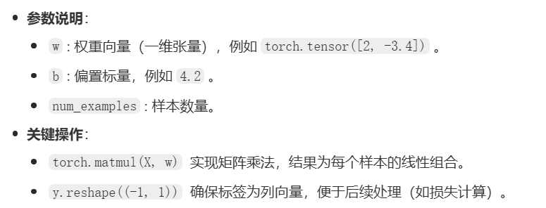
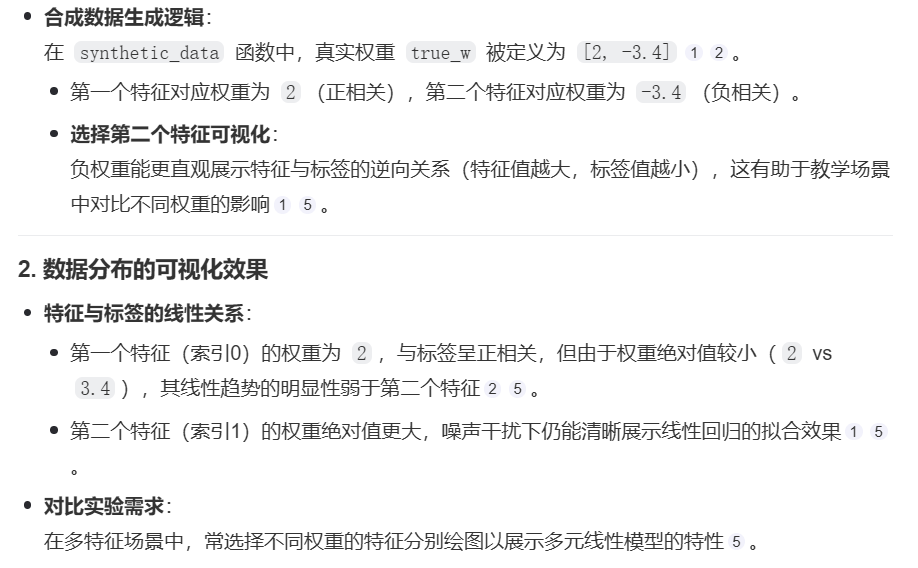
true_w = torch.tensor([2, -3.4])  # 定义真实权重
true_b = 4.2                      # 定义真实偏置
features, labels = synthetic_data(true_w, true_b, 1000)  # 生成1000个样本d2l.set_figsize()
d2l.plt.scatter(features[:, 1].detach().numpy(), labels.detach().numpy(), 1)

在这里插入图片描述
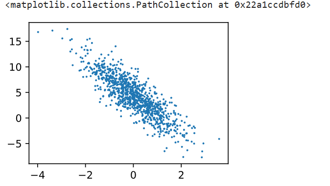
features[:, 1]: 选取所有样本的第二个特征（索引为1的列）。

3.2.1 读取数据集

def data_iter(batch_size, features, labels):num_examples = len(features)indices = list(range(num_examples))random.shuffle(indices)for i in range(0, num_examples, batch_size):batch_indices = torch.tensor(indices[i: min(i + batch_size, num_examples)])yield features[batch_indices], labels[batch_indices]batch_size = 10
for X, y in data_iter(batch_size, features, labels):print(X, '\n', y)break

tensor([[ 1.6556, 0.1851],
[-1.4880, 0.0684],
[ 1.0536, 0.9818],
[-0.7794, -1.9199],
[-0.3383, 0.2244],
[-0.2260, 3.1530],
[-2.3626, 1.1877],
[-0.3301, 0.1781],
[-0.6136, -1.2974],
[-0.3397, -0.2088]])
tensor([[ 6.8888],
[ 0.9887],
[ 2.9757],
[ 9.1748],
[ 2.7541],
[-6.9671],
[-4.5522],
[ 2.9436],
[ 7.3728],
[ 4.2270]])