当前位置：首页 > news >正文

基于有效样本数的类别平衡损失 (Class-Balanced Loss, CVPR 2019)

news 来源：原创 2025/4/20 9:00:25

Class-Balanced Loss Based on
Effective Number of Samples

Figure 1. Two classes, one from the head and one from the tail of a long-tailed dataset (iNaturalist 2017 [40] in this example), have drastically different number of samples. Models trained on these samples are biased toward dominant classes (black solid line). Reweighing the loss by inverse class frequency usually yields poor performance (red dashed line) on real-world data with high class imbalance. We propose a theoretical framework to quantify the effective number of samples by taking data overlap into consideration. A class-balanced term is designed to re-weight the loss by inverse effective number of samples. We show in experiments that the performance of a model can be improved when trained with the proposed class-balanced loss (blue dashed line).

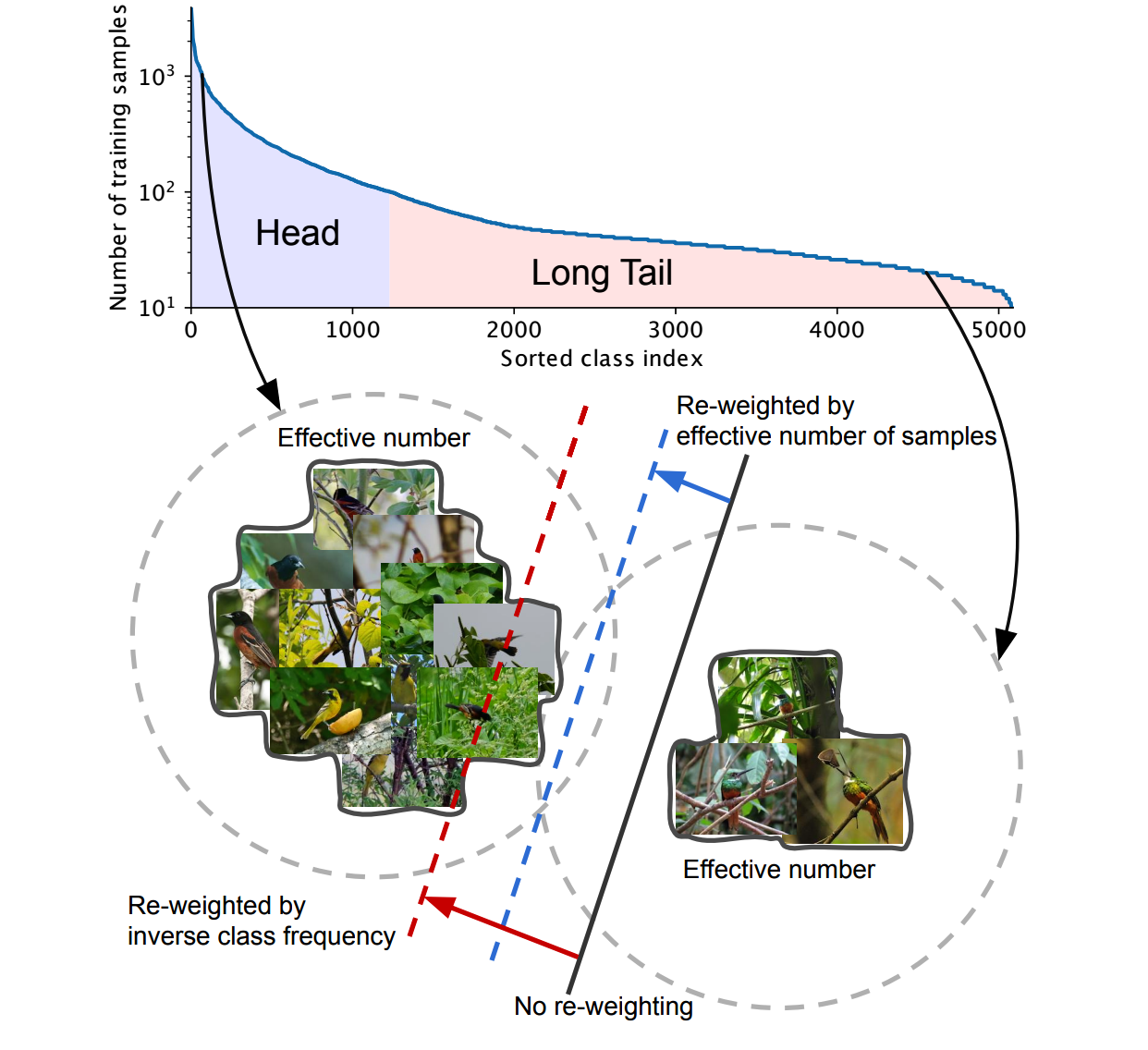
图1. 两个类别，一个来自长尾数据集（本例为iNaturalist 2017 [40]）的头部，一个来自尾部，样本数量差异巨大。在这些样本上训练的模型会偏向主导类别（黑色实线）。基于逆类别频率重新加权损失函数通常在高度类别不平衡的真实数据上表现不佳（红色虚线）。本文提出一个理论框架，通过考虑数据重叠来量化有效样本数量。设计了一个类别平衡项，通过逆有效样本数量对损失函数重新加权。实验表明，使用提出的类别平衡损失（蓝色虚线）训练时，模型性能可以得到提升。

Abstract

With the rapid increase of large-scale, real-world datasets, it becomes critical to address the problem of long-tailed data distribution (i.e., a few classes account for most of the data, while most classes are under-represented). Existing solutions typically adopt class re-balancing strategies such as re-sampling and re-weighting based on the number of observations for each class. In this work, we argue that as the number of samples increases, the additional benefit of a newly added data point will diminish. We introduce a novel theoretical framework to measure data overlap by associating with each sample a small neighboring region rather than a single point. The effective number of samples is defined as the volume of samples and can be calculated by a simple formula (1−β^n)/(1−β), where n is the number of samples and β ∈ [0, 1) is a hyperparameter. We design a re-weighting scheme that uses the effective number of samples for each class to re-balance the loss, thereby yielding a class-balanced loss. Comprehensive experiments are conducted on artificially induced long-tailed CIFAR datasets and large-scale datasets including ImageNet and iNaturalist. Our results show that when trained with the proposed class-balanced loss, the network is able to achieve significant performance gains on long-tailed datasets.

随着大规模真实数据集的快速增长，解决长尾数据分布问题（即少数类别占据大部分数据，而多数类别样本不足）变得至关重要。现有方案通常采用类别重平衡策略，如基于每类样本数量的重采样和重加权。

本文认为随着样本数量增加，新增数据点带来的边际收益会递减。

本文提出新颖的理论框架，通过将每个样本关联到一个小邻域而非单点来度量数据重叠。有效样本数量定义为样本体积，可通过简单公式(1−β^n)/(1−β)计算，其中n为样本数，β∈[0,1)是超参数。本文设计了重加权方案，利用每类的有效样本数量来重新平衡损失，从而得到类别平衡损失。

在人工构建的长尾CIFAR数据集和包括ImageNet、iNaturalist在内的大规模数据集上进行了全面实验。结果表明，使用提出的类别平衡损失训练时，网络能在长尾数据集上取得显著性能提升。

Introduction

The recent success of deep Convolutional Neural Networks (CNNs) for visual recognition [25, 36, 37, 16] owes much to the availability of large-scale, real-world annotated datasets [7, 27, 48, 40]. In contrast with commonly used visual recognition datasets (e.g., CIFAR [24, 39], ImageNet ILSVRC 2012 [7, 33] and CUB-200 Birds [42]) that exhibit roughly uniform distributions of class labels, real-world datasets have skewed [21] distributions, with a long-tail: a few dominant classes claim most of the examples, while most of the other classes are represented by relatively few examples. CNNs trained on such data perform poorly for weakly represented classes [19, 15, 41, 4].

A number of recent studies have aimed to alleviate the challenge of long-tailed training data [3, 31, 17, 41, 43, 12, 47, 44]. In general, there are two strategies: re-sampling and cost-sensitive re-weighting. In re-sampling, the number of examples is directly adjusted by over-sampling (adding repetitive data) for the minor class or under-sampling (removing data) for the major class, or both. In cost-sensitive re-weighting, we influence the loss function by assigning relatively higher costs to examples from minor classes. In the context of deep feature representation learning using CNNs, re-sampling may either introduce large amounts of duplicated samples, which slows down the training and makes the model susceptible to overfitting when oversampling, or discard valuable examples that are important for feature learning when under-sampling. Due to these disadvantages of applying re-sampling for CNN training, the present work focuses on re-weighting approaches, namely, how to design a better class-balanced loss.

深度卷积神经网络(CNN)在视觉识别中的成功很大程度上得益于大规模真实标注数据集。与常用视觉数据集的均匀类别分布不同，真实数据集具有偏态分布，呈现长尾特征：少数主导类别包含大多数样本，而其他多数类别样本稀少。在此类数据上训练的CNN对低代表性类别表现不佳。

近期多项研究致力于缓解长尾训练数据的挑战。主要策略分为重采样和代价敏感重加权。重采样通过为少数类过采样（添加重复数据）或对多数类欠采样（删除数据）来直接调整样本数量。代价敏感重加权则通过给少数类样本分配更高代价来影响损失函数。在CNN深度特征学习场景中，重采样可能引入大量重复样本导致训练速度下降和过拟合（过采样时），或丢失对特征学习至关重要的有价值样本（欠采样时）。鉴于重采样在CNN训练中的这些缺陷，本研究聚焦于重加权方法，即如何设计更好的类别平衡损失。

Typically, a class-balanced loss assigns sample weights inversely proportionally to the class frequency. This simple heuristic method has been widely adopted [17, 43]. However, recent work on training from large-scale, real-world, long-tailed datasets [30, 28] reveals poor performance when using this strategy. Instead, they use a "smoothed" version of weights that are empirically set to be inversely proportional to the square root of class frequency. These observations suggest an interesting question: how can we design a better class-balanced loss that is applicable to a diverse array of datasets?

通常，类别平衡损失会为样本分配与类别频率成反比的权重。这一简单启发式方法已被广泛采用。然而，最新针对大规模真实长尾数据集的研究表明，该策略会导致性能欠佳。研究者转而采用"平滑"权重，即经验性地设置为类别频率平方根的倒数。这些发现引出一个关键问题：如何设计更优的类别平衡损失，使其适用于多样化数据集？

We aim to answer this question from the perspective of sample size. As illustrated in Figure 1, we consider training a model to discriminate between a major class and a minor class from a long-tailed dataset. Due to highly imbalanced data, directly training the model or re-weighting the loss by inverse number of samples cannot yield satisfactory performance. Intuitively, the more data, the better. However, since there is information overlap among data, as the number of samples increases, the marginal benefit a model can extract from the data diminishes. In light of this, we propose a novel theoretical framework to characterize data overlap and calculate the effective number of samples in a model-and loss-agnostic manner. A class-balanced re-weighting term that is inversely proportional to the effective number of samples is added to the loss function. Extensive experimental results indicate that this class-balanced term provides a significant boost to the performance of commonly used loss functions for training CNNs on long-tailed datasets.

本文从样本规模视角解答该问题。如图1所示，考虑在长尾数据集中区分主导类和少数类时，高度不平衡的数据使得直接训练模型或采用样本数倒数加权均无法获得满意性能。虽然直觉认为数据越多越好，但由于数据间存在信息重叠，随着样本量增加，模型能从中获取的边际收益逐渐递减。为此，本文提出创新理论框架，以模型与损失无关的方式量化数据重叠并计算有效样本数量。通过在损失函数中添加与有效样本数成反比的类别平衡加权项，大量实验证明该方案能显著提升CNN在长尾数据集上的性能表现。

Our key contributions can be summarized as follows:
(1) We provide a theoretical framework to study the effective number of samples and show how to design a class-balanced term to deal with long-tailed training data.
(2) We show that significant performance improvements can be achieved by adding the proposed class-balanced term to existing commonly used loss functions including softmax cross-entropy, sigmoid cross-entropy and focal loss. In addition, we show our class-balanced loss can be used as a generic loss for visual recognition by outperforming commonly-used softmax cross-entropy loss on ILSVRC 2012. We believe our study on quantifying the effective number of samples and class-balanced loss can offer useful guidelines for researchers working in domains with long-tailed class distributions.

核心贡献包括：
(1) 建立理论框架研究有效样本数量，提出处理长尾训练数据的类别平衡项设计方法
(2) 证实将类别平衡项融入softmax交叉熵、sigmoid交叉熵和焦点损失等常用损失函数后，可获得显著性能提升。特别地，在ILSVRC 2012上，本文的类别平衡损失作为通用视觉识别损失，性能超越传统softmax交叉熵损失。关于有效样本量化与类别平衡损失的研究，为长尾类别分布领域研究者提供了实用指导。

Effective Number of Samples

We formulate the data sampling process as a simplified version of random covering. The key idea is to associate each sample with a small neighboring region instead of a single point. We present our theoretical framework and the formulation of calculating effective number of samples.

本文将数据采样过程建模为随机覆盖问题的简化版本。核心思想在于将每个样本关联到一个小邻域区域而非单个数据点。本节将阐述理论框架及有效样本数量的计算公式。

1. Data Sampling as Random Covering

Given a class, denote the set of all possible data in the feature space of this class as S. We assume the volume of S is N and N ≥ 1. Denote each data as a subset of S that has the unit volume of 1 and may overlap with other data. Consider the data sampling process as a random covering problem where each data (subset) is randomly sampled from S to cover the entire set of S. The more data is being sampled, the better the coverage of S is. The expected total volume of sampled data increases as the number of data increases and is bounded by N. Therefore, we define:

Definition 1 (Effective Number). The effective number of samples is the expected volume of samples.

1. 作为随机覆盖的数据采样

对于特定类别，设其特征空间中所有可能数据构成的集合为S。假设S的体积为N（N≥1），每个数据样本是S的子集且具有单位体积1，并可能与其他数据存在重叠。将数据采样过程视为随机覆盖问题：每次从S中随机采样一个数据子集以覆盖整个S集合。采样数据越多，S的覆盖率就越高。采样数据总体积的期望值随采样数量增加而增长，但上限为N。因此定义：

定义1（有效数量）：有效样本数量即样本的期望体积。

The calculation of the expected volume of samples is a very difficult problem that depends on the shape of the sample and the dimensionality of the feature space [18]. To make the problem tamable, we simplify the problem by not considering the situation of partial overlapping.

That is, we assume a newly sampled data can only interact with previously sampled data in two ways: either entirely inside the set of previously sampled data with the probability of p or entirely outside with the probability of 1−p, as illustrated in Figure 2. As the number of sampled data points increases, the probability p will be higher.

计算样本期望体积是极具挑战性的问题，其难度取决于样本形状和特征空间维度。为使问题可解，本文通过忽略部分重叠情况来简化模型。如图2所示，假设新采样数据与已采样数据的交互仅有两种方式：

完全包含在已采样数据集中（概率为p）
完全位于已采样数据集之外（概率为1-p）
如图2所示，随着采样数据点数量增加，重叠概率p将增大。

Figure 2. Giving the set of all possible data with volume N and the set of previously sampled data, a new sample with volume 1 has the probability of p being overlapped with previous data and the probability of 1 − p not being overlapped.

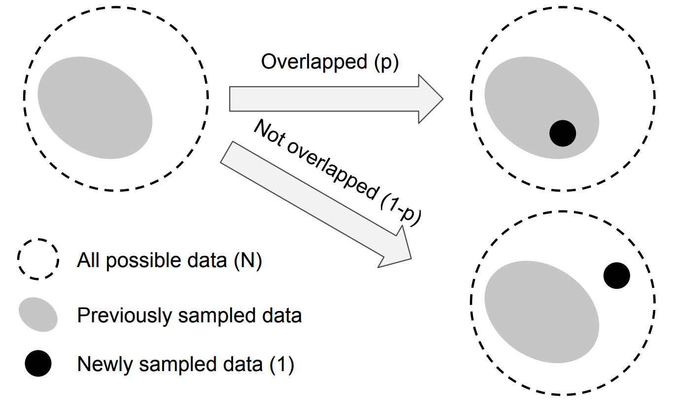
图2：给定体积为N的所有可能数据集合及已采样数据集，新采样的单位体积样本与已有数据发生重叠的概率为p，不重叠的概率为1-p。

Before we dive into the mathematical formulations, we discuss the connection between our definition of effective number of samples and real-world visual data. Our key idea is to capture the diminishing marginal benefits by using more data points of a class. Due to intrinsic similarities among real-world data, as the number of samples grows, it is highly possible that a newly added sample is a near-duplicate of existing samples. In addition, CNNs are trained with heavy data augmentations, where simple transformations such as random cropping, re-scaling and horizontal flipping will be applied to the input data. In this case, all augmented examples are also considered as same with the original example. Presumably, the stronger the data augmentation is, the smaller the N will be. The small neighboring region of a sample is a way to capture all near-duplicates and instances that can be obtained by data augmentation. For a class, N can be viewed as the number of unique prototypes.

在深入数学公式之前，首先探讨有效样本数量定义与现实视觉数据的关联。核心思想是通过使用更多同类数据点来捕捉边际效益递减现象。由于现实数据固有的相似性，随着样本量增加，新增样本极可能是已有样本的近似重复。此外，CNN训练采用强数据增强（如随机裁剪、缩放和水平翻转等基础变换），这些增强样本也被视为与原始样本等同。可以推断，数据增强越强，N值越小。样本的小邻域概念能够涵盖所有近似重复样本及通过数据增强获得的实例。对于某个类别，N可视为独特原型数量。

2. Mathematical Formulation

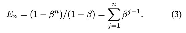
Denote the effective number (expected volume) of samples as E_n, where n ∈ ℤ>0 is the number of samples.

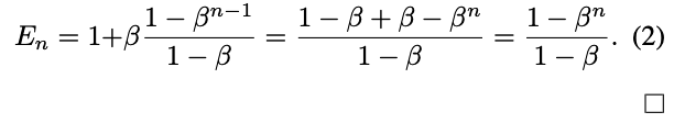
Proposition 1 (Effective Number). E_n = (1−βⁿ)/(1−β), where β = (N − 1)/N.

Proof. We prove the proposition by induction. It is obvious that E₁ = 1 because there is no overlapping. So E₁ = (1−β¹)/(1−β) = 1 holds. Now let's consider a general case where we have previously sampled n−1 examples and are about to sample the nᵗʰ example. Now the expected volume of previously sampled data is E_n-1 and the newly sampled data point has the probability of p = E_n-1/N to be overlapped with previous samples. Therefore, the expected volume after sampling nᵗʰ example is:

Assume holds, then

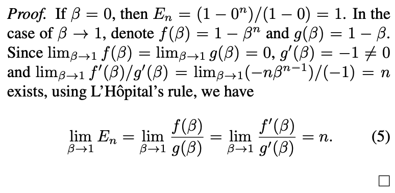
The above proposition shows that the effective number of samples is an exponential function of n. The hyperparameter β ∈ [0, 1) controls how fast E_n grows as n increases.

2. 数学表达

定义有效样本数量（期望体积）为E_n，其中n∈ℤ>0表示样本数。

命题1（有效数量）：E_n = (1−βⁿ)/(1−β), 其中 β = (N − 1)/N.

证明：采用数学归纳法。当n=1时显然E₁=1（无重叠），故E₁=(1−β¹)/(1−β)=1成立。现考虑一般情况：已采样n−1个样本时，已采样数据期望体积为E_n-1，新增第n个样本时，其与已有样本重叠概率p=E_n-1/N。因此采样第n个样本后期望体积为：

设成立，则

证毕。

该命题表明，有效样本数量是n的指数函数。超参数β∈[0,1)控制E_n随n增长的速度。

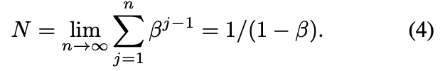
Another explanation of the effective number E_n is:

This means that the jᵗʰ sample contributes βʲ⁻¹ to the effective number. The total volume N for all possible data in the class can then be calculated as:

This is consistent with our definition of β in the proposition.

Implication 1 (Asymptotic Properties).

.

另一种解释：第j个样本对有效数量的贡献为

这意味着第 j 个样本对有效样本数量的贡献为βʲ⁻¹。因此，该类别所有可能数据的总体积N可通过以下极限计算得出：

证毕。

这与命题中对β的定义完全一致。

The asymptotic property of E_n shows that when N is large, the effective number of samples equals the actual number of samples n. In this scenario, we think the number of unique prototypes N is large, thus there is no data overlap and every sample is unique. On the other extreme, if N = 1, this means that we believe there exists a single prototype so that all the data in this class can be represented by this prototype via data augmentation, transformations, etc.

E_n的渐近特性表明，当N较大时，有效样本数量等于实际样本数n。这种情况下，本文认为独特原型数量N较大，因此不存在数据重叠且每个样本都是独特的。另一个极端情况是N=1，这意味着我们认为存在单一原型，该类所有数据都可通过数据增强、变换等方式由该原型表示。

Class-Balanced Loss

The Class-Balanced Loss is designed to address the problem of training from imbalanced data by introducing a weighting factor that is inversely proportional to the effective number of samples. The class-balanced loss term can be applied to a wide range of deep networks and loss functions. For an input sample x with label y ∈ {1, 2, . . . , C}, where C is the total number of classes, suppose the model's estimated class probabilities are , where pᵢ ∈ [0, 1] ∀ i, we denote the loss as L(p, y). Suppose the number of samples for class i is nᵢ, based on Equation 2, the proposed effective number of samples for class i is , where βᵢ = (Nᵢ − 1)/Nᵢ.

类别平衡损失

类别平衡损失旨在通过引入与有效样本数成反比的权重因子，解决不平衡数据训练问题。该类别平衡损失项可应用于多种深度网络和损失函数。对于输入样本x及其标签y∈{1,2,...,C}（C为类别总数），设模型预测的类别概率为p=[p₁,p₂,...,p_C]（pᵢ∈[0,1]），记损失函数为L(p,y)。若类别i的样本数为nᵢ，基于公式2，其有效样本数为E_{nᵢ}=(1−βᵢ^{nᵢ})/(1−βᵢ)，其中βᵢ=(Nᵢ−1)/Nᵢ。

Without further information of data for each class, it is difficult to empirically find a set of good hyperparameters Nᵢ for all classes. Therefore, in practice, we assume Nᵢ is only dataset-dependent and set Nᵢ = N, βᵢ = β = (N − 1)/N for all classes in a dataset. To balance the loss, we introduce a weighting factor αᵢ that is inversely proportional to the effective number of samples for class i: αᵢ ∝ 1/E_{nᵢ}. To make the total loss roughly in the same scale when applying αᵢ, we normalize αᵢ so that . For simplicity, we abuse the notation of 1/E_{nᵢ} to denote the normalized weighting factor in the rest of our paper.

由于缺乏各类别的先验信息，难以通过经验为所有类别设置理想的超参数Nᵢ。因此实践中，本文假设Nᵢ仅与数据集相关，统一设置Nᵢ=N，βᵢ=β=(N−1)/N。为实现损失平衡，本文引入权重因子αᵢ∝1/E_{nᵢ}，并将其归一化以保证总损失规模一致。为简化表示，后文中1/E_{nᵢ}均指归一化后的权重因子。

Formally speaking, given a sample from class i that contains nᵢ samples in total, we propose to add a weighting factor (1 − β)/(1 − β^{nᵢ}) to the loss function, with hyperparameter β ∈ [0, 1). The class-balanced (CB) loss can be written as:

where n_y is the number of samples in the ground-truth class y.

We visualize class-balanced loss in Figure 3 as a function of n_y for different β. Note that:

β = 0 corresponds to no re-weighting
β → 1 corresponds to re-weighing by inverse class frequency

对于包含nᵢ个样本的类别i中的样本，我们向损失函数添加权重因子(1−β)/(1−β^{nᵢ})（超参数β∈[0,1)）。类别平衡(CB)损失可表示为：

其中n_y表示真实类别y的样本数量。我们在图3中可视化了类别平衡损失随n_y变化的函数关系（针对不同β值）。需要特别说明的是：

β=0时，等价于不进行重新加权（原始损失函数）
β→1时，退化为按类别频率倒数进行重新加权

The proposed novel concept of effective number of samples enables us to use a hyperparameter β to smoothly adjust the class-balanced term between no re-weighting and re-weighing by inverse class frequency.

The proposed class-balanced term is:

Model-agnostic: Independent of the choice of model architecture
Loss-agnostic: Independent of the choice of loss function L and predicted class probabilities p

To demonstrate the proposed class-balanced loss is generic, we show how to apply the class-balanced term to three commonly used loss functions: Softmax cross-entropy loss；Sigmoid cross-entropy loss；Focal loss.

提出的有效样本数新概念使我们能够通过超参数β在不重新加权和按类别频率倒数重新加权之间平滑调整类别平衡项。

提出的类别平衡项具有以下特性：

模型无关性：独立于模型架构的选择
损失函数无关性：不受损失函数L和预测类别概率p的选择影响

为证明提出的类别平衡损失的通用性，我们展示了如何将该平衡项应用于三种常用损失函数：

Softmax交叉熵损失
Sigmoid交叉熵损失
Focal损失

1. Class-Balanced Softmax Cross-Entropy Loss

Suppose the predicted output from the model for all classes are , where C is the total number of classes. The softmax function regards each class as mutually exclusive and calculates the probability distribution over all classes as {1, 2, ..., C}. Given a sample with class label y, the softmax cross-entropy (CE) loss for this sample is written as:

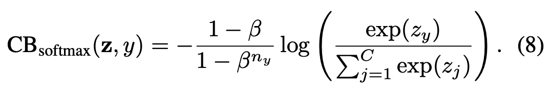
Suppose class y has n_y training samples, the class-balanced (CB) softmax cross-entropy loss is:

1. 类别平衡的Softmax交叉熵损失

假设模型对所有类别的预测输出为z = [z₁, z₂, ..., z_C]（C为类别总数）。Softmax函数将每个类别视为互斥的，并计算所有类别的概率分布为pᵢ = e^{zᵢ}/∑_{j=1}^C e^{zⱼ}（i ∈ {1,2,...,C}）。给定类别标签y的样本，其Softmax交叉熵(CE)损失表示为：

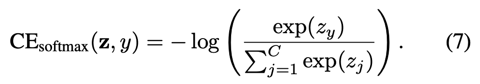
若类别y有n_y个训练样本，则类别平衡(CB)的Softmax交叉熵损失为：

2. Class-Balanced Sigmoid Cross-Entropy Loss

Different from softmax, class-probabilities calculated by sigmoid function assume each class is independent and not mutually exclusive. When using sigmoid function, we regard multi-class visual recognition as multiple binary classification tasks, where each output node of the network is performing a one-vs-all classification to predict the probability of the target class over the rest of classes. Compared with softmax, sigmoid presumably has two advantages for real-world datasets:

Sigmoid doesn't assume mutual exclusiveness among classes, which aligns well with real-world data, where classes might have fine-grained similarities, especially in cases with large numbers of classes.
Since each class is considered independent and has its own predictor, sigmoid unifies single-label classification with multi-label prediction. This is particularly valuable for real-world data which often contains multiple semantic labels.

2. 类别平衡的Sigmoid交叉熵损失

与Softmax不同，Sigmoid函数计算的类别概率假设各类别是独立且非互斥的。使用Sigmoid函数时，我们将多类别视觉识别视为多个二分类任务，网络的每个输出节点执行一对多分类，预测目标类别相对于其他类别的概率。相比Softmax，Sigmoid对真实数据集具有两大优势：

Sigmoid不假设类别互斥性，这与真实数据特性相符，特别是当存在大量具有细粒度相似性的类别时
由于每个类别被视为独立的且拥有独立的预测器，Sigmoid统一了单标签与多标签预测，这对常包含多重语义标签的真实数据尤为重要

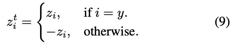
Using the same notations as softmax cross-entropy, for simplicity, we define z^t_i as:

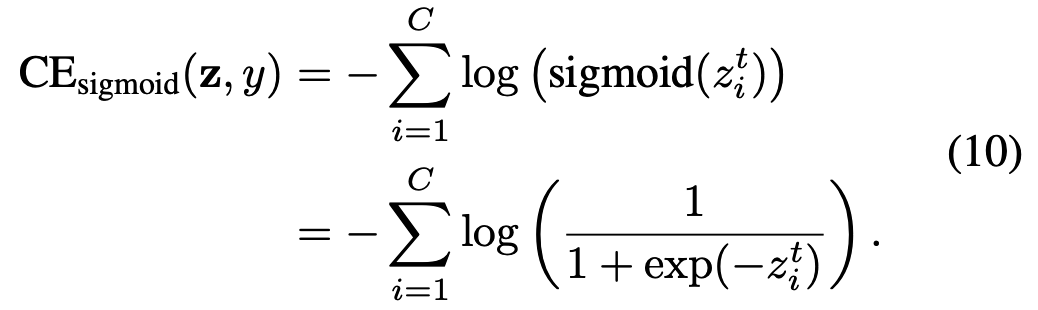
Then the sigmoid cross-entropy (CE) loss can be written as:

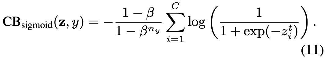
The class-balanced (CB) sigmoid cross-entropy loss is:

沿用Softmax交叉熵的符号表示，为简化定义z^t_i为：

则Sigmoid交叉熵损失(CE)可表示为：

对应的类别平衡(CB) Sigmoid交叉熵损失为：

3. Class-Balanced Focal Loss

The recently proposed focal loss (FL) [26] adds a modulating factor to the sigmoid cross-entropy loss to:

Reduce relative loss for well-classified samples
Focus on difficult samples

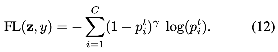
Denote p^t_i = sigmoid(z^t_i) = 1/(1 + exp(−z^t_i)), the focal loss can be written as:

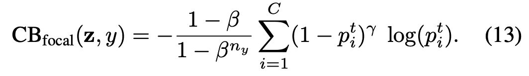
The class-balanced (CB) focal loss is:

The original focal loss has an α-balanced variant. The class-balanced focal loss is same as α-balanced focal loss when . Therefore, the class-balanced term can be viewed as an explicit way to set α_t in focal loss based on the effective number of samples.