大语言模型时代，单细胞注释也需要集思广益（mLLMCelltype）

生信碱移

LLM细胞注释

mLLMCelltype 是一款基于多种大语言模型的共识聚类方法，在多项数据测试中，实现了最高精度的细胞类型鉴定。

细胞类型注释是单细胞RNA测序（scRNA-seq）数据分析中的关键步骤。目前注释方法的金标准依赖于人工专家，需要手动将每个细胞簇中高表达的基因与文献中的经典细胞类型标记基因进行比对。尽管如此，这一流程及其耗时，而且需要专业的生物知识。随着测序成本的下降，当数据集规模扩大到数百万个来自不同组织的细胞，手动注释的方法已变得难以实现。

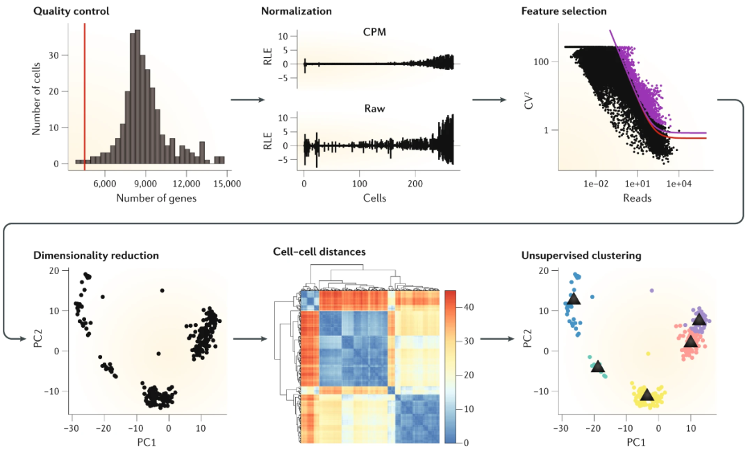
▲ 单细胞分析常规流程如上：之前分享过一篇单细胞的聚类方法，包括像近期发表的一篇集成随机森林 NM 方法其实算是延续之作，这个领域其实可选择的工具很多，并没有说一定要跑常规的流程。点击此处阅读

先前的一些研究人员提出监督学习方法（如SingleR）、无监督学习方法（如scCATCH）以及基于知识的方法（如CellAssign）用于单细胞数据的细胞类型注释。尽管有许多算法被提出，注释准确性仍然远未达到理想状态，尤其是在研究较少的组织类型中特别明显。新兴的模型利用大语言模型与集成学习方法提取或整合多维度注释信息，具有代表的是 popV 和 GPTCelltype。前者基于集成学习的思想，整合多个单一注释工具的优势；而后者则利用大语言模型（LLM）的能力，结合LLM训练数据中蕴含的先验生物学知识，给出有生物学依据的细胞类型注释。

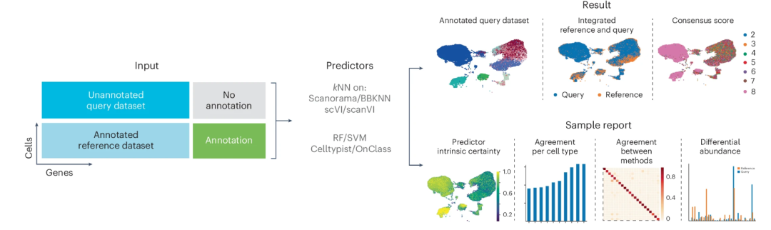
▲ 单细胞 popV 注释算法：PopV 将未标注的查询数据集和已标注的参考数据集作为输入。每种专家算法都会预测查询数据集上的标签，从而得出细胞类型注释。通过对这些方法的一致性进行评分，可以量化各自标签转移的确定性。DOI: 10.1038/s41588-024-01993-3。如果你十分感兴趣单细胞领域的算法进展，推荐点击此处阅读另一篇文章。

尽管如此，目前最先进的方法依然存在显著的局限性。考虑到不同的大型语言模型具有互补潜力，来自美国德克萨斯州大学的研究人员提出了一种多LLM共识迭代模型框架 mLLMCelltype。顾名思义，该框架通过整合多个 LLM 模型以实现 scRNA-seq 的细胞类型一致性注释。在涵盖 26 种组织、超过 800 万个细胞的 50 个多样化数据集上，mLLMCelltype以平均准确率（77.3%对 61.3%）领先最佳现有方法近15%。mLLMCelltype提供R语言或Python两种调用方式，不存在平台迁移成本，大家可以看看。

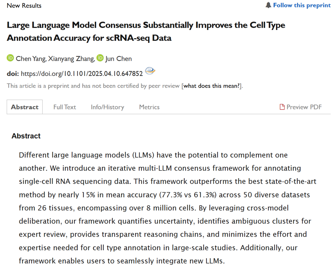
▲ DOI: 10.1101/2025.04.10.647852。

mLLMCelltype 框架工作流程如下图所示。本文简要介绍其使用，感兴趣的铁子可以自行阅读学习其原文与github仓：

• https://github.com/cafferychen777/mLLMCelltype

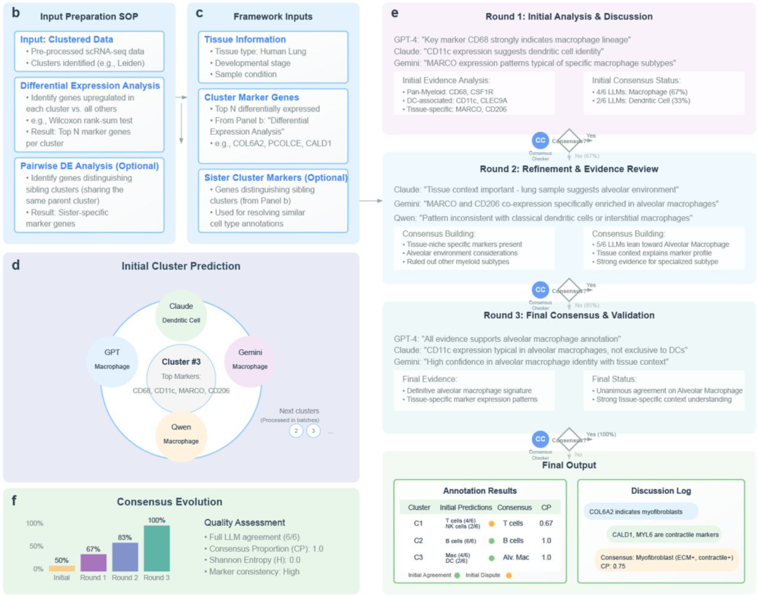
▲ 图：mLLMCelltype 工作流程。① 首先，通过差异表达分析识别出每个细胞簇的标记基因，随后结合组织上下文信息，构成下一步的输入 (图b-c)；② 随后，多个大语言模型（LLMs）独立接收这些输入，并为每个细胞簇提出初步的细胞类型注释，同时基于标记基因证据提供生物学推理 (图d,e)。对于那些未能立即达成高共识的细胞簇，框架将启动一个迭代审议流程 (图e)；③ 在每一轮协商中，LLMs 会共享其结构化的论据，讨论特定标记基因的重要性（例如泛髓系标记 CD68 与组织特异性标记 MARCO 的对比）、潜在参与的信号通路，并评估组织上下文对细胞身份的影响(图e)；④ 每个 LLM 会根据其他模型呈现的证据和推理结果，重新权衡并优化自己的分类结果(图e)；⑤ 在每轮审议之后，由一个专门的共识检查模型（Consensus Checker LLM）对参与模型之间的意见一致程度进行评估，并与预设的共识阈值进行比较（mLLMCelltype 的关键点, 图e）。如果达成共识，则流程终止，输出最终注释结果及对应的置信评分；如果未达成共识，则进入下一轮讨论（最多允许若干轮），或将该细胞簇标记为模糊不清。

0.软件安装

① 在R语言中安装：

devtools::install_github("cafferychen777/mLLMCelltype", subdir = "R")

② 或在python中安装：

pip install mllmcelltype

需要注意的是，mLLMCelltype支持以下模型：

• OpenAI: GPT-4.1/GPT-4.5/GPT-4o (API Key)

• Anthropic: Claude-3.7-Sonnet/Claude-3.5-Haiku (API Key)

• Google: Gemini-2.0-Pro/Gemini-2.0-Flash (API Key)

• Alibaba: Qwen2.5-Max (API Key)

• DeepSeek: DeepSeek-V3/DeepSeek-R1 (API Key)

• Minimax: MiniMax-Text-01 (API Key)

• Stepfun: Step-2-16K (API Key)

• Zhipu: GLM-4 (API Key)

• X.AI: Grok-3/Grok-3-mini (API Key)

1.基于scanpy的注释流程

① 读入单细胞数据，进行常规上游流程（标准化/高变基因筛选/线性降维/邻居图构建/细胞聚类）

import scanpy as sc
import pandas as pd
from mllmcelltype import annotate_clusters, setup_logging, interactive_consensus_annotation
import os# 设置记录信息
setup_logging()# 加载数据
adata = sc.read_h5ad('your_data.h5ad')# 检查提供的数据时候进行了上游流程，如果无则使用默认流程与leiden进行聚类：
if'leiden'notin adata.obs.columns:print("Computing leiden clustering...")if'log1p'notin adata.uns:sc.pp.normalize_total(adata, target_sum=1e4)sc.pp.log1p(adata)if'X_pca'notin adata.obsm:sc.pp.highly_variable_genes(adata, min_mean=0.0125, max_mean=3, min_disp=0.5)sc.pp.pca(adata, use_highly_variable=True)sc.pp.neighbors(adata, n_neighbors=10, n_pcs=30)sc.tl.leiden(adata, resolution=0.8)print(f"Leiden clustering completed, found {len(adata.obs['leiden'].cat.categories)} clusters")

② 鉴定不同分群的标志基因，在scanpy中一般使用rank_genes_groups函数：

sc.tl.rank_genes_groups(adata, 'leiden', method='wilcoxon')# 提取基因作为一个字典，需要保证此时adata.var.index为基因名称
marker_genes = {}
for i in range(len(adata.obs['leiden'].cat.categories)):genes = [adata.uns['rank_genes_groups']['names'][str(i)][j] for j in range(10)]marker_genes[str(i)] = genes

③ 设置模型API，有些模型的 api 还是比较难用上的，毕竟是国外的：

os.environ["OPENAI_API_KEY"] = "your-openai-api-key"      # Required for GPT models
os.environ["ANTHROPIC_API_KEY"] = "your-anthropic-api-key"  # Required for Claude models
os.environ["GEMINI_API_KEY"] = "your-gemini-api-key"      # Required for Gemini models
os.environ["QWEN_API_KEY"] = "your-qwen-api-key"        # Required for Qwen models
# 下方为其它选项
# os.environ["DEEPSEEK_API_KEY"] = "your-deepseek-api-key"   # For DeepSeek models
# os.environ["ZHIPU_API_KEY"] = "your-zhipu-api-key"       # For GLM models
# os.environ["STEPFUN_API_KEY"] = "your-stepfun-api-key"    # For Step models
# os.environ["MINIMAX_API_KEY"] = "your-minimax-api-key"    # For MiniMax models

④ 进行多个模型的共识注释：

consensus_results = interactive_consensus_annotation(marker_genes=marker_genes,species="human",tissue="blood",models=["gpt-4o", "claude-3-7-sonnet-20250219", "gemini-1.5-pro", "qwen-max-2025-01-25"],consensus_threshold=1,  # Adjust threshold for consensus agreementmax_discussion_rounds=3   # Maximum rounds of discussion between models
)

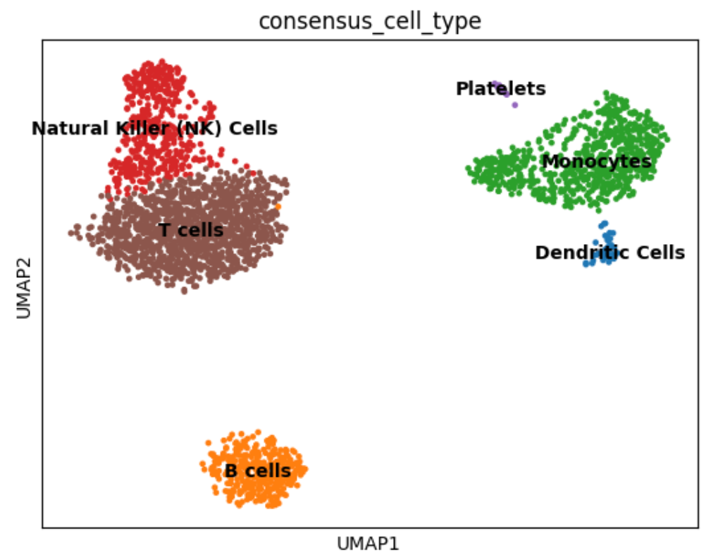
⑤ 获得最终结果，并进行可视化：

# Access the final consensus annotations from the dictionary
final_annotations = consensus_results["consensus"]# Add consensus annotations to your AnnData object
adata.obs['consensus_cell_type'] = adata.obs['leiden'].astype(str).map(final_annotations)# Add uncertainty metrics to your AnnData object
adata.obs['consensus_proportion'] = adata.obs['leiden'].astype(str).map(consensus_results["consensus_proportion"])
adata.obs['entropy'] = adata.obs['leiden'].astype(str).map(consensus_results["entropy"])# IMPORTANT: Ensure UMAP coordinates are calculated before visualization
# If UMAP coordinates are not available in your AnnData object, compute them:
if'X_umap'notin adata.obsm:print("Computing UMAP coordinates...")# Make sure neighbors are computed firstif'neighbors'notin adata.uns:sc.pp.neighbors(adata, n_neighbors=10, n_pcs=30)sc.tl.umap(adata)print("UMAP coordinates computed")# Visualize results with enhanced aesthetics
# Basic visualization
sc.pl.umap(adata, color='consensus_cell_type', legend_loc='right', frameon=True, title='mLLMCelltype Consensus Annotations')# More customized visualization
import matplotlib.pyplot as plt# Set figure size and style
plt.rcParams['figure.figsize'] = (10, 8)
plt.rcParams['font.size'] = 12# Create a more publication-ready UMAP
fig, ax = plt.subplots(1, 1, figsize=(12, 10))
sc.pl.umap(adata, color='consensus_cell_type', legend_loc='on data', frameon=True, title='mLLMCelltype Consensus Annotations',palette='tab20', size=50, legend_fontsize=12, legend_fontoutline=2, ax=ax)# Visualize uncertainty metrics
fig, (ax1, ax2) = plt.subplots(1, 2, figsize=(16, 7))
sc.pl.umap(adata, color='consensus_proportion', ax=ax1, title='Consensus Proportion',cmap='viridis', vmin=0, vmax=1, size=30)
sc.pl.umap(adata, color='entropy', ax=ax2, title='Annotation Uncertainty (Shannon Entropy)',cmap='magma', vmin=0, size=30)
plt.tight_layout()

2.基于Seurat的注释流程

Seurat 上使用这个软件的流程是一模一样的，区别仅仅只是在于解释器环境：

① 读入单细胞数据，进行常规上游流程（标准化/高变基因筛选/线性降维/邻居图构建/细胞聚类）

library(mLLMCelltype)
library(Seurat)
library(dplyr)
library(ggplot2)
library(cowplot) # Added for plot_grid# 加载数据
pbmc <- readRDS("your_seurat_object.rds")# 可以选择进行常规流程
# pbmc <- NormalizeData(pbmc)
# pbmc <- FindVariableFeatures(pbmc, selection.method = "vst", nfeatures = 2000)
# pbmc <- ScaleData(pbmc)
# pbmc <- RunPCA(pbmc)
# pbmc <- FindNeighbors(pbmc, dims = 1:10)
# pbmc <- FindClusters(pbmc, resolution = 0.5)
# pbmc <- RunUMAP(pbmc, dims = 1:10)

② 鉴定不同分群的标志基因，在seurat中一般使用FindAllMarkers函数：

pbmc_markers <- FindAllMarkers(pbmc,only.pos = TRUE,min.pct = 0.25,logfc.threshold = 0.25)
# 设置缓存路径
cache_dir <- "./mllmcelltype_cache"
dir.create(cache_dir, showWarnings = FALSE, recursive = TRUE)

③ 设置模型API，并进行多个模型的共识注释：

consensus_results <- interactive_consensus_annotation(input = pbmc_markers,tissue_name = "human PBMC",  # provide tissue contextmodels = c("claude-3-7-sonnet-20250219",  # Anthropic"gpt-4o",                   # OpenAI"gemini-1.5-pro",           # Google"qwen-max-2025-01-25"       # Alibaba),api_keys = list(anthropic = "your-anthropic-key",openai = "your-openai-key",gemini = "your-google-key",qwen = "your-qwen-key"),top_gene_count = 10,controversy_threshold = 1.0,entropy_threshold = 1.0,cache_dir = cache_dir
)

④ 获得最终结果，并进行可视化：

# Print structure of results to understand the data
print("Available fields in consensus_results:")
print(names(consensus_results))# Add annotations to Seurat object
# Get cell type annotations from consensus_results$final_annotations
cluster_to_celltype_map <- consensus_results$final_annotations# Create new cell type identifier column
cell_types <- as.character(Idents(pbmc))
for (cluster_id in names(cluster_to_celltype_map)) {cell_types[cell_types == cluster_id] <- cluster_to_celltype_map[[cluster_id]]
}# Add cell type annotations to Seurat object
pbmc$cell_type <- cell_types# Add uncertainty metrics
# Extract detailed consensus results containing metrics
consensus_details <- consensus_results$initial_results$consensus_results# Create a data frame with metrics for each cluster
uncertainty_metrics <- data.frame(cluster_id = names(consensus_details),consensus_proportion = sapply(consensus_details, function(res) res$consensus_proportion),entropy = sapply(consensus_details, function(res) res$entropy)
)# Add uncertainty metrics for each cell
pbmc$consensus_proportion <- uncertainty_metrics$consensus_proportion[match(current_clusters, uncertainty_metrics$cluster_id)]
pbmc$entropy <- uncertainty_metrics$entropy[match(current_clusters, uncertainty_metrics$cluster_id)]# Save results for future use
saveRDS(consensus_results, "pbmc_mLLMCelltype_results.rds")
saveRDS(pbmc, "pbmc_annotated.rds")# Visualize results with SCpubr for publication-ready plots
if (!requireNamespace("SCpubr", quietly = TRUE)) {remotes::install_github("enblacar/SCpubr")
}
library(SCpubr)
library(viridis)  # For color palettes# Basic UMAP visualization with default settings
pdf("pbmc_basic_annotations.pdf", width=8, height=6)
SCpubr::do_DimPlot(sample = pbmc,group.by = "cell_type",label = TRUE,legend.position = "right") +ggtitle("mLLMCelltype Consensus Annotations")
dev.off()# More customized visualization with enhanced styling
pdf("pbmc_custom_annotations.pdf", width=8, height=6)
SCpubr::do_DimPlot(sample = pbmc,group.by = "cell_type",label = TRUE,label.box = TRUE,legend.position = "right",pt.size = 1.0,border.size = 1,font.size = 12) +ggtitle("mLLMCelltype Consensus Annotations") +theme(plot.title = element_text(hjust = 0.5))
dev.off()# Visualize uncertainty metrics with enhanced SCpubr plots
# Get cell types and create a named color palette
cell_types <- unique(pbmc$cell_type)
color_palette <- viridis::viridis(length(cell_types))
names(color_palette) <- cell_types# Cell type annotations with SCpubr
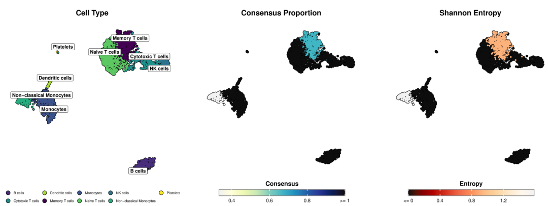
p1 <- SCpubr::do_DimPlot(sample = pbmc,group.by = "cell_type",label = TRUE,legend.position = "bottom",  # Place legend at the bottompt.size = 1.0,label.size = 4,  # Smaller label font sizelabel.box = TRUE,  # Add background box to labels for better readabilityrepel = TRUE,  # Make labels repel each other to avoid overlapcolors.use = color_palette,plot.title = "Cell Type") +theme(plot.title = element_text(hjust = 0.5, margin = margin(b = 15, t = 10)),legend.text = element_text(size = 8),legend.key.size = unit(0.3, "cm"),plot.margin = unit(c(0.8, 0.8, 0.8, 0.8), "cm"))# Consensus proportion feature plot with SCpubr
p2 <- SCpubr::do_FeaturePlot(sample = pbmc,features = "consensus_proportion",order = TRUE,pt.size = 1.0,enforce_symmetry = FALSE,legend.title = "Consensus",plot.title = "Consensus Proportion",sequential.palette = "YlGnBu",  # Yellow-Green-Blue gradient, following Nature Methods standardssequential.direction = 1,  # Light to dark directionmin.cutoff = min(pbmc$consensus_proportion),  # Set minimum valuemax.cutoff = max(pbmc$consensus_proportion),  # Set maximum valuena.value = "lightgrey") +  # Color for missing valuestheme(plot.title = element_text(hjust = 0.5, margin = margin(b = 15, t = 10)),plot.margin = unit(c(0.8, 0.8, 0.8, 0.8), "cm"))# Shannon entropy feature plot with SCpubr
p3 <- SCpubr::do_FeaturePlot(sample = pbmc,features = "entropy",order = TRUE,pt.size = 1.0,enforce_symmetry = FALSE,legend.title = "Entropy",plot.title = "Shannon Entropy",sequential.palette = "OrRd",  # Orange-Red gradient, following Nature Methods standardssequential.direction = -1,  # Dark to light direction (reversed)min.cutoff = min(pbmc$entropy),  # Set minimum valuemax.cutoff = max(pbmc$entropy),  # Set maximum valuena.value = "lightgrey") +  # Color for missing valuestheme(plot.title = element_text(hjust = 0.5, margin = margin(b = 15, t = 10)),plot.margin = unit(c(0.8, 0.8, 0.8, 0.8), "cm"))# Combine plots with equal widths
pdf("pbmc_uncertainty_metrics.pdf", width=18, height=7)
combined_plot <- cowplot::plot_grid(p1, p2, p3, ncol = 3, rel_widths = c(1.2, 1.2, 1.2))
print(combined_plot)
dev.off()

这个工具给大家推荐一手

各位老铁关注起来