Python----深度学习(基于深度学习Pytroch簇分类,圆环分类,月牙分类)
一、引言
深度学习的重要性
深度学习是一种通过模拟人脑神经元结构来进行数据学习和模式识别的技术,在分类任务中展现出强大的能力。
分类任务的多样性
分类任务涵盖了各种场景,例如簇分类、圆环分类和月牙分类,每种任务都有不同的特征和应用。
二、分类任务详解
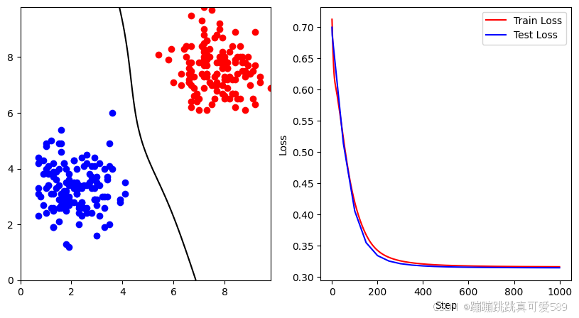
2.1、簇分类
- 定义
簇分类旨在将数据点分为多个簇或类别,目标是在特征空间中找到数据点的天然聚集。 - 数据特性
通常数据聚集在不同的区域形成簇,这些簇可能具有不同的形状和大小。 - 应用场景
数据挖掘、市场细分、社交网络分析等。
簇分类数据
class1_points = np.array([[3.2, 3.0], [2.6, 3.4], [3.5, 4.9], [2.5, 3.4], [1.8, 2.7], [1.3, 1.9], [1.1, 3.4], [1.0, 4.0],[1.2, 5.0], [2.8, 4.1],[2.7, 3.1], [2.6, 4.5], [2.1, 3.3], [2.3, 2.4], [2.6, 3.1], [1.9, 3.0], [0.7, 4.2], [1.4, 3.3],[1.6, 4.6], [2.3, 2.0],[1.3, 4.2], [1.9, 3.8], [3.6, 6.0], [1.2, 3.1], [1.6, 3.1], [3.5, 4.1], [1.7, 2.6], [2.4, 3.3],[0.8, 2.2], [1.5, 4.3],[1.3, 3.9], [1.6, 5.4], [3.4, 3.7], [2.3, 3.4], [2.6, 2.4], [1.8, 2.5], [1.1, 4.1], [1.8, 2.8],[0.7, 4.4], [1.1, 3.4],[1.9, 3.6], [1.5, 4.9], [1.0, 3.3], [1.4, 3.6], [2.8, 3.3], [3.1, 4.2], [2.7, 3.8], [3.3, 2.6],[3.0, 2.7], [0.8, 3.0],[1.1, 3.8], [1.8, 3.5], [1.9, 2.8], [0.7, 3.1], [2.5, 2.6], [1.3, 2.5], [2.9, 2.9], [3.1, 2.3],[2.4, 2.8], [1.5, 4.0],[1.2, 3.8], [2.4, 2.3], [2.1, 1.9], [2.6, 4.2], [2.1, 2.8], [1.6, 2.6], [0.9, 3.8], [1.5, 2.1],[1.7, 3.0], [3.0, 2.9],[2.3, 2.6], [1.5, 2.9], [2.9, 2.9], [1.9, 2.7], [0.9, 2.7], [1.0, 4.9], [3.3, 4.0], [2.3, 2.7],[2.2, 4.0], [1.7, 4.2],[1.5, 3.4], [2.1, 3.5], [2.7, 3.9], [1.0, 4.8], [2.4, 2.8], [1.5, 2.6], [2.2, 3.2], [2.5, 2.6],[3.9, 2.8], [2.9, 4.1],[2.1, 4.3], [1.9, 3.4], [1.3, 1.9], [0.7, 3.3], [1.8, 4.2], [1.7, 3.2], [3.9, 2.9], [1.6, 4.2],[2.4, 4.4], [1.8, 1.3],[3.5, 2.0], [2.2, 3.1], [3.0, 3.5], [2.9, 3.3], [1.9, 2.9], [1.6, 2.7], [2.8, 3.6], [3.0, 2.7],[2.9, 4.4], [3.1, 3.4],[1.9, 1.2], [3.0, 1.6], [2.0, 3.7], [1.3, 3.1], [2.8, 2.4], [1.5, 2.6], [2.2, 3.1], [3.0, 3.7],[0.9, 4.3], [3.4, 3.6],[1.0, 2.4], [2.1, 3.3], [0.7, 2.3], [2.9, 2.3], [2.7, 3.5], [1.3, 2.6], [1.7, 4.2], [2.5, 4.1],[2.2, 3.4], [3.3, 3.0],[2.2, 3.5], [1.7, 3.1], [1.9, 2.8], [1.7, 2.9], [3.4, 3.0], [1.6, 4.9], [2.8, 3.7], [1.3, 3.7],[2.6, 2.6], [4.1, 3.5],[4.1, 3.1], [1.2, 2.6], [2.5, 3.0], [1.8, 4.0], [3.6, 4.0], [2.1, 4.3], [1.8, 3.2], [3.3, 1.9],[2.4, 3.5], [1.4, 3.9]])
class2_points = np.array([[8.8, 7.2], [7.8, 7.3], [6.8, 7.8], [8.1, 7.5], [7.8, 5.4], [7.6, 8.1], [8.3, 7.5], [6.9, 8.5],[8.0, 8.2], [8.7, 7.2],[8.8, 7.0], [8.2, 8.3], [7.7, 7.6], [8.3, 8.1], [8.3, 7.7], [8.0, 7.7], [6.7, 6.2], [8.4, 7.8],[7.6, 7.3], [6.4, 8.3],[8.0, 6.6], [7.0, 6.1], [8.2, 6.5], [6.7, 6.4], [7.1, 8.4], [6.6, 7.6], [7.9, 7.6], [8.0, 8.0],[7.3, 8.6], [8.7, 7.5],[7.8, 9.2], [7.3, 6.1], [7.7, 7.4], [8.0, 7.3], [8.2, 7.3], [6.5, 8.4], [6.7, 7.0], [7.9, 8.2],[6.0, 7.1], [7.9, 7.6],[7.1, 7.8], [9.0, 7.4], [7.2, 8.5], [9.1, 6.5], [7.3, 8.6], [7.2, 7.7], [8.8, 7.3], [7.0, 6.5],[6.7, 8.4], [7.4, 8.3],[9.2, 6.3], [7.8, 8.0], [9.4, 7.3], [8.0, 6.5], [6.8, 7.3], [8.5, 7.4], [6.6, 7.4], [8.6, 8.4],[9.8, 6.9], [6.7, 9.5],[6.5, 8.0], [8.1, 7.6], [7.4, 8.0], [8.8, 6.1], [7.1, 9.3], [7.3, 7.7], [7.9, 6.7], [7.2, 9.8],[8.7, 7.8], [7.8, 9.0],[7.2, 7.3], [9.2, 8.9], [7.3, 7.3], [8.3, 6.7], [7.2, 8.2], [8.1, 7.6], [7.5, 9.7], [6.8, 6.9],[8.8, 7.5], [7.6, 7.0],[7.9, 8.7], [8.8, 7.8], [7.5, 7.0], [8.2, 8.2], [6.9, 6.7], [8.1, 7.8], [8.9, 7.4], [9.4, 7.1],[5.8, 7.9], [7.2, 8.0],[8.0, 7.2], [7.2, 9.0], [7.3, 7.4], [7.3, 7.9], [9.0, 7.0], [7.9, 7.8], [7.2, 6.9], [8.4, 6.7],[8.4, 6.2], [8.4, 7.9],[7.6, 6.5], [6.3, 7.0], [8.1, 7.2], [7.2, 7.9], [7.9, 7.0], [7.7, 7.0], [7.1, 7.4], [8.9, 7.7],[7.5, 6.3], [7.3, 7.4],[8.1, 6.9], [5.4, 8.1], [7.7, 7.1], [7.8, 7.8], [7.3, 8.1], [9.1, 7.5], [7.4, 7.1], [6.6, 7.2],[7.7, 7.8], [7.7, 8.8],[6.5, 8.4], [8.5, 8.0], [5.9, 8.3], [6.9, 6.4], [7.7, 6.8], [8.5, 6.5], [8.6, 6.5], [8.4, 7.2],[8.0, 7.9], [8.3, 8.4],[9.2, 7.7], [8.6, 8.0], [7.2, 8.3], [7.6, 8.7], [6.7, 7.5], [6.6, 7.1], [8.7, 8.0], [7.0, 7.8],[8.4, 8.9], [6.6, 7.8],[8.3, 6.7], [6.7, 7.8], [6.6, 7.1], [8.3, 7.2], [8.9, 8.0], [6.8, 6.6], [8.0, 7.7], [6.3, 7.4],[7.2, 8.8], [7.7, 7.4]])
模型训练效果
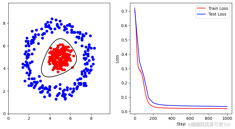
2.2、圆环分类
- 定义
圆环分类任务涉及在特征空间中识别环形结构的数据分布。 - 数据特性
数据点围绕某个中心形成多个同心圆,每个环对应不同的类别。 - 应用场景
图像分类、手写数字识别、模式识别等。
圆环分类数据
class1_points = np.array([[1.7, 4.6], [5.4, 7.7], [3.8, 1.9], [3.5, 2.2], [2.2, 2.5], [4.1, 8.1], [3.7, 7.3], [1.8, 4.2],[6.8, 2.7], [6.9, 3.1],[7.9, 6.9], [8.1, 5.0], [7.2, 7.0], [7.9, 3.8], [6.3, 2.2], [5.0, 2.6], [4.9, 7.6], [6.1, 1.6],[3.0, 6.6], [3.3, 6.7],[1.8, 4.9], [3.2, 7.5], [7.8, 3.7], [7.3, 2.5], [7.1, 6.7], [1.6, 6.0], [2.6, 2.8], [1.9, 4.3],[2.5, 2.8], [7.3, 3.3],[7.7, 5.1], [2.7, 7.4], [6.2, 7.7], [5.6, 7.6], [6.4, 7.2], [7.1, 6.6], [3.8, 8.1], [2.4, 6.3],[7.5, 3.7], [1.6, 2.9],[3.9, 7.8], [7.2, 6.9], [7.4, 4.8], [7.5, 4.4], [2.0, 5.2], [2.0, 4.0], [7.3, 3.8], [5.5, 7.6],[7.5, 5.9], [4.0, 2.4],[6.9, 7.1], [5.3, 2.0], [3.3, 7.0], [4.0, 2.3], [2.7, 2.7], [5.9, 7.8], [5.7, 2.1], [7.8, 5.9],[2.6, 7.0], [5.4, 2.1],[7.0, 2.7], [5.4, 7.4], [7.0, 6.4], [7.5, 5.3], [4.2, 2.1], [3.7, 7.7], [7.7, 5.3], [6.1, 7.3],[1.6, 4.3], [3.3, 2.4],[1.9, 6.4], [1.9, 6.2], [7.7, 6.0], [4.2, 8.4], [4.7, 1.6], [3.0, 3.3], [2.1, 3.6], [1.8, 6.7],[4.8, 7.7], [6.8, 2.7],[3.3, 2.5], [5.6, 7.5], [5.9, 7.9], [2.3, 4.6], [2.2, 6.2], [4.8, 1.7], [1.9, 4.2], [1.4, 4.1],[3.5, 7.1], [5.9, 7.8],[6.6, 6.8], [2.3, 5.3], [4.0, 7.6], [3.9, 7.2], [4.6, 2.4], [3.0, 2.2], [7.3, 2.7], [1.6, 5.3],[2.8, 2.8], [2.5, 5.7],[7.7, 5.6], [4.6, 1.3], [3.1, 7.3], [2.0, 3.1], [7.1, 3.7], [6.1, 7.7], [3.1, 1.9], [6.5, 6.3],[2.1, 3.6], [7.3, 5.2],[1.7, 6.0], [2.2, 5.0], [7.4, 2.7], [2.2, 6.4], [5.0, 8.2], [2.6, 2.8], [2.6, 2.5], [7.5, 4.0],[1.7, 3.7], [3.8, 7.7],[2.9, 6.2], [4.9, 1.8], [1.9, 5.3], [6.8, 6.7], [5.2, 1.6], [5.7, 2.3], [3.8, 8.1], [6.7, 3.0],[2.3, 3.1], [8.3, 5.8],[2.1, 4.5], [5.3, 1.7], [3.2, 1.9], [7.0, 3.1], [6.3, 2.0], [4.2, 7.2], [6.1, 7.4], [2.3, 6.5],[5.4, 1.5], [5.7, 7.2],[4.5, 7.5], [2.4, 6.8], [7.6, 4.5], [3.3, 2.0], [1.8, 3.6], [1.8, 4.3], [7.5, 4.9], [4.6, 8.3],[6.9, 6.8], [7.4, 3.4],[3.6, 7.9], [7.6, 4.4], [7.8, 6.1], [6.0, 2.2], [6.4, 2.7], [4.9, 7.6], [1.7, 6.4], [7.7, 5.7],[6.8, 6.8], [3.1, 2.9],[2.0, 2.5], [4.5, 2.3], [6.7, 7.2], [7.5, 7.1], [1.9, 5.5], [5.5, 1.7], [6.6, 2.2], [6.1, 7.2],[3.9, 2.1], [2.5, 6.6],[7.7, 3.9], [7.4, 5.5], [7.6, 3.8], [3.7, 2.2], [2.3, 7.3], [5.0, 2.2], [5.5, 1.4], [2.9, 7.0],[6.7, 2.4], [2.0, 5.6],[6.4, 2.6], [7.3, 4.9], [4.0, 1.6], [3.3, 2.3], [7.6, 5.1], [3.5, 1.5], [4.7, 7.9], [6.1, 7.4],[2.2, 6.2], [6.9, 2.6],[2.2, 2.7], [4.1, 7.5], [8.2, 4.4], [3.5, 7.8], [2.4, 6.5], [2.1, 3.8], [1.8, 5.1], [2.3, 2.6],[6.4, 2.7], [7.0, 2.6],[7.4, 3.6], [5.9, 1.7], [8.3, 5.8], [7.8, 3.6], [7.7, 5.1], [8.0, 3.9], [1.3, 5.3], [3.4, 7.1],[4.7, 7.8], [2.1, 3.8],[7.1, 6.0], [7.5, 4.1], [7.1, 3.5], [7.3, 6.9], [6.6, 2.3], [7.5, 3.3], [7.1, 6.5], [8.0, 5.8],[8.0, 4.2], [3.6, 7.7],[1.9, 5.0], [2.6, 2.8], [5.1, 7.0], [6.9, 7.2], [2.0, 6.0], [7.5, 2.5], [4.0, 2.1], [2.9, 7.0],[4.2, 7.2], [5.3, 1.8],[2.6, 6.8], [3.1, 2.3], [3.6, 2.3], [5.5, 1.3], [1.3, 4.2], [6.2, 1.9], [2.5, 3.1], [1.8, 4.5],[1.7, 5.5], [5.7, 7.8],[8.2, 4.8], [2.0, 3.4], [1.4, 4.4], [5.5, 7.9], [4.0, 1.7], [7.8, 4.7], [6.3, 7.2], [2.5, 2.3],[7.4, 4.4], [5.1, 7.9]])
class2_points = np.array([[5.7, 4.8], [4.8, 5.0], [4.7, 4.6], [4.6, 5.3], [5.0, 5.5], [4.3, 4.9], [4.2, 5.9], [6.0, 5.0],[4.1, 5.2], [5.4, 5.0],[4.9, 5.4], [4.5, 6.2], [5.3, 5.5], [4.2, 5.0], [4.0, 4.9], [5.9, 4.9], [4.3, 6.1], [4.5, 4.3],[5.1, 5.8], [5.6, 4.5],[4.9, 4.3], [5.5, 5.7], [5.4, 5.0], [4.7, 4.9], [5.6, 5.3], [5.8, 4.8], [4.8, 5.6], [5.3, 5.3],[5.1, 4.7], [5.0, 5.3],[4.0, 4.4], [5.9, 5.2], [5.7, 4.7], [5.8, 5.2], [5.1, 4.0], [5.8, 5.9], [5.3, 6.0], [5.5, 4.8],[5.1, 4.7], [4.7, 4.3],[5.7, 5.0], [4.3, 4.7], [5.7, 4.9], [4.7, 4.0], [4.9, 4.9], [5.2, 4.6], [4.6, 5.6], [5.2, 5.3],[4.8, 5.9], [4.5, 4.7],[5.3, 5.2], [4.7, 4.3], [4.7, 5.7], [4.7, 4.2], [4.7, 5.3], [5.3, 5.4], [5.4, 5.9], [4.6, 4.1],[4.1, 5.8], [5.6, 5.1],[5.2, 4.5], [5.6, 4.7], [5.0, 4.8], [5.7, 4.3], [4.5, 5.7], [4.4, 5.7], [5.5, 5.3], [4.7, 5.4],[5.1, 5.7], [5.2, 4.3],[4.6, 4.9], [4.7, 5.5], [4.5, 4.2], [5.2, 4.5], [5.4, 3.9], [4.0, 5.0], [4.4, 4.0], [5.0, 4.2],[5.8, 5.6], [5.8, 5.2],[4.7, 4.6], [4.7, 5.8], [5.6, 4.5], [5.8, 4.9], [4.6, 5.5], [5.6, 4.5], [5.1, 4.5], [4.2, 4.8],[4.9, 5.3], [5.0, 5.2],[4.0, 4.8], [5.5, 4.8], [6.0, 4.7], [4.4, 5.1], [4.3, 4.9], [5.1, 5.6], [4.7, 5.6], [5.1, 4.9],[4.2, 5.4], [4.4, 4.6],[5.5, 5.9], [4.1, 4.8], [5.0, 4.6], [5.2, 5.0], [4.1, 5.5], [4.6, 5.1], [5.2, 5.5], [5.1, 4.0],[4.4, 4.5], [5.3, 5.3],[4.8, 5.3], [5.2, 4.6], [5.7, 4.4], [4.3, 5.0], [5.1, 4.9], [4.6, 5.0], [5.4, 5.6], [5.3, 4.4],[4.6, 4.3], [5.2, 5.6],[5.0, 4.3], [4.4, 4.4], [5.5, 4.9], [4.3, 5.5], [5.0, 5.3], [4.8, 4.9], [5.3, 5.6], [4.1, 4.7],[4.6, 5.2], [5.5, 4.6],[4.6, 4.6], [4.5, 5.4], [4.6, 4.2], [5.1, 4.3], [5.2, 4.3], [5.1, 5.6], [5.5, 4.5], [5.1, 4.0],[4.5, 5.1], [4.8, 3.7],[4.3, 5.1], [4.6, 5.4], [5.2, 3.9], [4.6, 5.1], [4.2, 5.1], [4.5, 5.2], [5.6, 5.3], [5.6, 5.1],[5.9, 5.2], [5.0, 4.1],[5.1, 4.3], [4.8, 6.0], [5.3, 5.5], [5.3, 4.4], [4.4, 5.1], [5.2, 5.0], [4.9, 4.4], [5.3, 5.2],[5.2, 6.1], [5.6, 5.9],[4.7, 4.2], [6.1, 5.6], [4.6, 5.7], [5.5, 5.0], [4.5, 5.1], [4.8, 6.0], [4.8, 5.0], [5.5, 4.3],[4.1, 4.9], [3.9, 4.6],[4.9, 5.3], [4.4, 4.1], [4.6, 5.3], [5.0, 4.7], [5.3, 5.9], [5.1, 5.4], [5.3, 5.3], [4.9, 4.5],[5.6, 5.1], [5.2, 4.5],[5.3, 4.6], [5.5, 5.6], [5.0, 6.1], [4.5, 5.3], [4.8, 5.6], [4.7, 4.9], [4.7, 5.6], [4.6, 4.3],[5.8, 5.0], [4.9, 4.8],[5.6, 5.3], [5.5, 5.2], [4.8, 5.3], [4.6, 4.5], [5.2, 4.9], [5.5, 5.6], [6.2, 4.1], [5.6, 5.3],[5.3, 5.4], [5.4, 5.0],[5.5, 4.8], [5.1, 4.6], [4.8, 5.4], [4.8, 5.3], [5.8, 4.8], [4.5, 4.8], [4.6, 4.9], [4.3, 3.9],[4.6, 5.3], [5.1, 5.3],[5.4, 5.7], [4.3, 5.2], [4.8, 4.9], [5.6, 4.7], [4.2, 5.0], [5.3, 5.6], [4.9, 4.0], [5.1, 4.7],[5.0, 5.4], [6.0, 5.5],[5.5, 4.6], [5.7, 5.3], [4.5, 4.7], [5.5, 5.0], [5.9, 4.9], [5.5, 4.6], [4.9, 5.6], [5.4, 5.3],[5.2, 4.4], [4.3, 4.5],[5.1, 4.2], [4.3, 5.1], [5.6, 5.7], [4.8, 5.0], [5.1, 5.5], [5.7, 5.2], [5.9, 4.9], [5.1, 4.3],[5.3, 5.2], [4.4, 4.7],[5.2, 5.8], [6.3, 5.1], [4.0, 5.4], [5.4, 4.7], [4.2, 5.3], [5.7, 4.9], [5.4, 5.5], [4.8, 5.2],[5.4, 5.8], [4.6, 5.0]])
模型训练效果
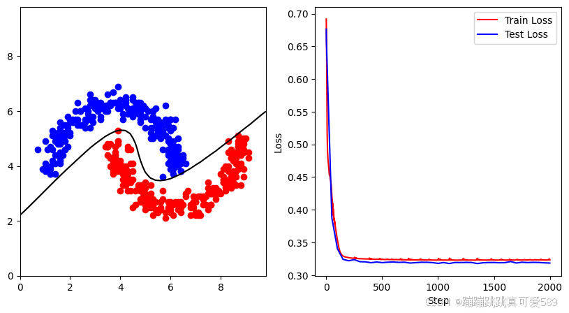
2.3、月牙分类
- 定义
月牙分类任务要求识别流形或不规则的形状,数据分布呈现出像月牙形状的特征。 - 数据特性
数据集中的点通常呈现出一种弯曲的形态,具有独特的边界。 - 应用场景
生物医学影像分析、信号处理、推荐系统等。
月牙分类数据
class1_points = np.array([[6.5, 4.3], [4.5, 6.4], [1.3, 5.1], [1.7, 4.4], [4.8, 5.7], [5.4, 5.6], [1.8, 4.9], [1.2, 3.8],[2.8, 5.7], [6.4, 3.8],[4.5, 5.9], [5.3, 6.0], [5.9, 5.0], [1.7, 4.6], [2.3, 5.7], [3.4, 6.1], [5.9, 4.4], [5.4, 5.1],[5.2, 5.2], [5.6, 5.4],[4.2, 6.2], [1.4, 3.7], [3.6, 6.3], [4.8, 6.0], [4.8, 6.0], [5.0, 6.1], [5.8, 5.1], [1.6, 4.5],[1.5, 5.1], [2.2, 6.0],[5.1, 5.8], [3.8, 6.3], [2.0, 5.7], [2.1, 5.6], [2.0, 5.1], [1.0, 4.9], [3.0, 6.3], [6.0, 4.2],[2.3, 6.3], [4.8, 6.1],[1.8, 5.1], [2.2, 5.7], [6.3, 4.3], [5.7, 5.3], [5.6, 5.5], [3.0, 6.1], [6.1, 3.7], [6.3, 4.7],[3.4, 6.1], [5.2, 5.7],[5.8, 3.7], [0.7, 4.6], [4.9, 6.2], [1.8, 5.1], [4.6, 5.9], [1.5, 5.0], [1.4, 4.4], [4.0, 6.4],[5.3, 5.8], [4.6, 6.1],[3.5, 6.0], [6.2, 4.6], [4.5, 6.0], [2.6, 6.1], [5.9, 5.0], [2.8, 6.4], [2.4, 6.0], [5.3, 6.0],[2.0, 5.7], [1.2, 3.7],[2.8, 5.9], [2.5, 5.5], [6.3, 4.6], [1.2, 3.7], [6.3, 4.4], [6.0, 4.8], [1.5, 4.2], [6.4, 4.2],[1.3, 4.6], [2.0, 5.2],[1.9, 5.2], [1.6, 5.4], [5.5, 5.7], [3.5, 6.6], [1.7, 5.0], [6.2, 4.6], [6.1, 4.5], [4.1, 5.9],[6.1, 4.9], [1.7, 5.2],[3.5, 6.2], [2.9, 6.4], [5.0, 5.8], [2.5, 5.8], [3.1, 6.0], [2.0, 5.1], [2.6, 5.7], [6.1, 4.0],[6.5, 4.4], [5.4, 6.1],[5.9, 4.1], [4.7, 5.9], [2.4, 6.5], [4.5, 6.4], [5.9, 4.6], [0.9, 3.9], [3.6, 6.3], [3.7, 6.3],[1.6, 4.3], [6.0, 5.7],[4.2, 6.3], [1.8, 5.2], [2.7, 5.9], [2.4, 5.5], [6.4, 3.8], [5.2, 6.1], [6.2, 4.7], [4.2, 6.5],[5.7, 3.6], [3.9, 6.1],[1.1, 4.6], [5.5, 5.3], [2.0, 5.9], [5.2, 5.4], [5.7, 5.2], [5.3, 5.0], [1.4, 4.1], [2.8, 6.6],[3.6, 6.3], [1.1, 4.3],[5.5, 5.2], [3.9, 6.9], [6.2, 4.2], [5.5, 5.5], [1.6, 4.1], [1.1, 3.9], [1.4, 4.9], [4.5, 6.1],[1.7, 5.0], [1.9, 4.7],[5.8, 5.7], [4.8, 5.6], [3.2, 5.7], [6.3, 4.0], [1.6, 4.2], [1.8, 5.1], [1.9, 5.5], [2.9, 5.6],[1.0, 3.8], [5.9, 5.5],[2.6, 5.6], [5.3, 5.4], [1.5, 5.0], [3.2, 6.1], [1.0, 4.1], [1.9, 5.8], [3.3, 6.2], [6.1, 3.9],[2.9, 5.8], [4.8, 5.9],[6.0, 4.4], [3.6, 6.2], [1.6, 5.1], [5.6, 5.0], [4.0, 6.2], [6.2, 4.3], [4.2, 6.4], [4.0, 6.1],[5.5, 5.1], [4.3, 6.1],[4.5, 5.8], [3.7, 6.7], [1.6, 5.6], [5.7, 4.6], [1.6, 4.9], [6.2, 5.7], [2.8, 6.2], [2.1, 5.7],[5.8, 6.2], [1.5, 5.0],[5.6, 5.6], [4.1, 5.7], [1.8, 4.6], [6.4, 4.1], [1.2, 3.8], [2.4, 6.0], [1.5, 5.2], [6.0, 3.9],[5.9, 4.7], [1.9, 5.5],[2.3, 5.5], [6.1, 4.4], [2.0, 5.2], [1.8, 5.5], [4.6, 6.3], [3.4, 6.2], [4.7, 6.3], [3.1, 6.1],[3.8, 6.3], [5.7, 5.5],[1.9, 5.4], [4.7, 5.9], [6.0, 4.2], [4.5, 6.5], [1.3, 4.2], [5.1, 6.0], [1.8, 5.2], [4.0, 6.4],[5.8, 5.6], [1.2, 3.9],[6.1, 5.4], [1.7, 4.9], [6.3, 5.0], [5.2, 5.0], [3.0, 6.4], [1.6, 4.8], [1.5, 5.2], [4.7, 6.3],[1.5, 4.8], [5.3, 5.8],[4.3, 5.9], [3.2, 6.3], [2.4, 5.5], [2.6, 5.4], [1.2, 3.9], [4.8, 6.3], [6.2, 4.6], [1.3, 5.3],[6.6, 4.1], [2.9, 6.3],[3.3, 6.1], [6.0, 5.3], [1.5, 4.9], [5.6, 5.7], [5.9, 4.5], [4.9, 6.1], [6.0, 4.6], [5.0, 5.4],[3.4, 6.1], [5.9, 4.9],[2.8, 5.4], [1.9, 5.3], [3.2, 5.8], [1.2, 4.7], [3.1, 6.3], [1.2, 4.0], [6.0, 5.7], [2.7, 6.0],[3.4, 6.0], [5.9, 5.4]])
class2_points = np.array([[6.5, 2.5], [6.4, 2.3], [6.6, 2.8], [7.0, 2.6], [4.3, 2.9], [4.1, 3.7], [3.9, 3.3], [7.2, 2.7],[3.8, 4.5], [4.0, 4.7],[4.0, 3.9], [8.3, 3.8], [6.5, 3.1], [8.0, 3.6], [7.9, 3.4], [6.8, 2.5], [4.0, 4.4], [7.0, 2.6],[7.7, 3.1], [6.0, 2.1],[6.7, 2.7], [8.7, 4.2], [4.0, 3.9], [5.9, 2.2], [6.3, 2.7], [7.3, 2.9], [5.0, 2.6], [8.1, 3.9],[4.2, 4.0], [5.1, 2.5],[8.2, 3.3], [7.1, 2.9], [5.0, 3.0], [7.1, 2.3], [4.8, 3.1], [3.5, 4.4], [8.3, 3.3], [5.2, 3.0],[6.1, 2.2], [6.8, 2.2],[3.9, 4.9], [8.6, 3.6], [6.0, 2.3], [4.1, 4.0], [5.2, 2.8], [8.2, 3.5], [8.1, 3.4], [8.7, 4.9],[5.0, 2.4], [5.0, 2.6],[8.0, 3.0], [8.4, 4.3], [5.3, 2.7], [8.7, 5.1], [5.6, 2.5], [5.4, 2.7], [3.8, 4.5], [9.1, 4.3],[8.8, 4.1], [4.7, 3.3],[8.4, 4.6], [8.3, 4.5], [7.0, 2.7], [6.4, 2.3], [5.2, 2.5], [7.0, 2.2], [8.6, 3.3], [7.5, 3.0],[4.0, 3.9], [7.6, 3.0],[7.0, 2.7], [4.3, 3.1], [5.7, 2.8], [3.8, 4.3], [4.9, 3.1], [4.1, 3.3], [7.0, 2.3], [5.1, 2.9],[8.9, 4.5], [6.0, 2.7],[7.4, 2.6], [8.7, 4.7], [8.6, 4.5], [7.7, 3.0], [8.9, 5.0], [4.1, 4.0], [3.9, 4.8], [3.7, 3.8],[5.5, 2.3], [7.5, 3.4],[4.2, 3.3], [4.1, 3.5], [7.8, 3.1], [3.8, 4.7], [5.2, 3.3], [3.5, 4.7], [3.5, 4.8], [3.9, 4.2],[6.7, 3.1], [7.9, 3.0],[8.6, 4.1], [8.5, 4.4], [7.3, 2.6], [3.4, 4.7], [8.7, 3.9], [7.6, 3.0], [4.6, 3.1], [4.8, 2.7],[4.5, 2.5], [7.4, 2.9],[5.1, 2.7], [6.9, 2.7], [7.6, 2.6], [9.0, 5.0], [7.1, 2.2], [5.0, 2.7], [5.6, 2.4], [3.6, 4.8],[6.0, 2.4], [6.9, 2.9],[8.3, 4.9], [3.9, 4.0], [4.9, 3.1], [8.7, 3.9], [6.3, 2.4], [6.8, 2.5], [5.8, 2.1], [4.5, 4.1],[4.7, 3.2], [6.3, 2.6],[8.8, 4.8], [8.6, 4.1], [4.5, 3.8], [3.6, 4.3], [8.8, 5.0], [4.2, 3.9], [8.6, 4.4], [8.8, 4.0],[5.0, 3.4], [6.4, 2.5],[4.6, 2.6], [6.0, 2.6], [8.1, 3.5], [8.7, 4.5], [4.8, 2.8], [5.9, 2.7], [6.8, 2.6], [8.9, 4.6],[6.4, 2.6], [6.9, 2.5],[8.8, 3.3], [3.7, 4.0], [8.3, 4.0], [3.6, 4.3], [7.2, 2.2], [8.8, 4.4], [8.7, 4.7], [3.8, 4.4],[8.1, 3.4], [3.5, 4.7],[8.7, 4.1], [4.3, 3.8], [3.6, 4.0], [5.0, 2.7], [7.7, 3.2], [8.4, 3.2], [4.3, 3.7], [8.6, 4.3],[7.5, 3.2], [8.3, 3.8],[4.9, 2.9], [5.4, 2.4], [3.9, 4.9], [8.9, 3.6], [8.3, 3.4], [8.2, 3.3], [7.8, 2.8], [8.2, 3.2],[8.9, 4.8], [8.6, 3.8],[3.9, 5.3], [4.4, 4.6], [7.8, 3.0], [6.9, 2.7], [7.7, 3.0], [3.7, 3.7], [6.6, 3.0], [5.3, 2.6],[4.4, 4.1], [8.1, 3.6],[8.5, 3.4], [8.0, 3.7], [5.2, 2.7], [7.3, 2.8], [4.1, 4.0], [8.5, 3.6], [7.5, 2.4], [3.9, 3.8],[5.9, 2.5], [6.6, 2.9],[4.4, 3.4], [4.8, 3.3], [4.4, 3.1], [8.7, 4.8], [6.2, 2.7], [5.0, 3.2], [5.6, 2.7], [8.5, 4.2],[4.2, 3.5], [4.0, 3.1],[3.8, 4.1], [5.3, 2.2], [4.9, 3.3], [5.7, 3.1], [4.4, 3.5], [5.3, 2.8], [4.2, 3.3], [8.4, 3.6],[8.1, 3.5], [3.8, 4.4],[3.6, 4.3], [4.3, 4.6], [7.9, 3.1], [8.9, 4.9], [7.8, 3.2], [4.1, 3.7], [4.8, 3.1], [3.7, 4.3],[8.5, 3.8], [5.2, 2.7],[7.3, 2.8], [6.5, 2.6], [8.4, 4.3], [8.2, 4.0], [7.2, 2.9], [3.7, 4.2], [7.6, 2.6], [4.3, 4.7],[4.5, 3.5], [4.0, 4.2],[6.4, 2.7], [6.3, 2.6], [8.9, 3.9], [5.8, 2.3], [6.1, 2.6], [4.1, 3.7], [8.2, 3.1], [9.1, 4.5],[3.7, 4.1], [6.3, 2.7]])
模型训练效果
三、PyTorch实现
以月牙分类为例
划分数据集
# 将 point1 分割为训练集和测试集
np.random.shuffle(class1_points)  # 随机打乱数据
split_index = int(0.1 * len(class1_points))  # 取前 10% 的数据作为测试集class1_train_points = class1_points[split_index:]
class2_train_points = class2_points[split_index:]
class1_test_points = class1_points[:split_index]
class2_test_points = class2_points[:split_index]# 合并两类点
train_points = np.concatenate((class1_train_points, class2_train_points))
# 标签 0表示类别1,1表示类别2
train_labels1 = np.zeros(len(class1_train_points))
train_labels2 = np.ones(len(class2_train_points))
train_labels = np.concatenate((train_labels1, train_labels2))
# 合并两类点
test_points = np.concatenate((class1_test_points, class2_test_points))
# 标签 0表示类别1,1表示类别2
test_labels1 = np.zeros(len(class1_test_points))
test_labels2 = np.ones(len(class2_test_points))
test_labels = np.concatenate((test_labels1, test_labels2))
构建模型
class ModelClass(nn.Module):def __init__(self):super().__init__()self.layer1 = nn.Linear(2, 8)self.layer2 = nn.Linear(8, 16)self.layer3 = nn.Linear(16, 32)self.layer4 = nn.Linear(32, 16)self.layer5 = nn.Linear(16, 8)self.layer6 = nn.Linear(8, 2)def forward(self, x):x = torch.tanh(self.layer1(x))x = torch.tanh(self.layer2(x))x = torch.tanh(self.layer3(x))x = torch.tanh(self.layer4(x))x = torch.tanh(self.layer5(x))x = torch.softmax(self.layer6(x),dim=1)return xmodel = ModelClass()创建损失函数和优化器
criterion = nn.CrossEntropyLoss()
optimizer = optim.Adam(model.parameters(), lr=0.01, weight_decay=0.005)
模型训练
for n in range(1,2001):# 将numpy数据转换为torch tensorinputs = torch.tensor(train_points, dtype=torch.float32)train_labels = torch.tensor(train_labels, dtype=torch.long)# 前向传播outputs = model(inputs)loss = criterion(outputs, train_labels)# 反向传播和优化optimizer.zero_grad()loss.backward()optimizer.step()if n % 100== 0 or n == 1:print(n,loss.item())可视化
# 创建等高线绘图的网格点
x_min, x_max = 0, 10
y_min, y_max = 0, 10
step_size = 0.2
xx, yy = np.meshgrid(np.arange(x_min, x_max, step_size),np.arange(y_min, y_max, step_size))
grid_points = np.c_[xx.ravel(), yy.ravel()]# 创建三维图形和右侧的二维子图
fig = plt.figure(figsize=(10, 5))ax1 = fig.add_subplot(121)
ax2 = fig.add_subplot(122)step_list = []
loss_list = []
test_step_list = []
test_loss_list = []# 开始迭代
for n in range(1,2001):# 将numpy数据转换为torch tensorinputs = torch.tensor(train_points, dtype=torch.float32)train_labels = torch.tensor(train_labels, dtype=torch.long)# 前向传播outputs = model(inputs)loss = criterion(outputs, train_labels)# 反向传播和优化optimizer.zero_grad()loss.backward()optimizer.step()# 更新右侧的损失图数据并绘制step_list.append(n)loss_list.append(loss.detach())# 显示频率设置frequency_display = 50# 显示与输出if n % 100== 0 or n == 1:# 使用训练好的模型预测网格点的标签grid_points_tensor = torch.tensor(grid_points, dtype=torch.float32)Z = model(grid_points_tensor).detach().numpy()Z = Z[:, 1]  # 取正类的概率值Z = Z.reshape(xx.shape)# 绘制2D图ax1 = plt.subplot(121)ax1.clear()ax1.scatter(class1_train_points[:, 0], class1_train_points[:, 1], c='blue', label='label1')ax1.scatter(class2_train_points[:, 0], class2_train_points[:, 1], c='red', label='label2')ax1.contour(xx, yy, Z, levels=[0.5], colors='black')# 计算测试集损失test_inputs = torch.tensor(test_points, dtype=torch.float32)y_pred_test = model(test_inputs)test_labels = torch.tensor(test_labels, dtype=torch.long)loss_test = criterion(y_pred_test, test_labels)test_step_list.append(n)test_loss_list.append(loss_test.detach())ax2 = plt.subplot(122)ax2.clear()ax2.plot(step_list, loss_list, 'r-', label='Train Loss')ax2.plot(test_step_list, test_loss_list, 'b-', label='Test Loss')  # 绘制测试集损失ax2.set_xlabel("Step")ax2.set_ylabel("Loss")ax2.legend()plt.show()
完整代码
import numpy as np
import torch
import random
import torch.nn as nn
import torch.optim as optim
import matplotlib.pyplot as plt
import torch.nn.init as init# 创造数据,数据集
class1_points = np.array([[6.5, 4.3], [4.5, 6.4], [1.3, 5.1], [1.7, 4.4], [4.8, 5.7], [5.4, 5.6], [1.8, 4.9], [1.2, 3.8],[2.8, 5.7], [6.4, 3.8],[4.5, 5.9], [5.3, 6.0], [5.9, 5.0], [1.7, 4.6], [2.3, 5.7], [3.4, 6.1], [5.9, 4.4], [5.4, 5.1],[5.2, 5.2], [5.6, 5.4],[4.2, 6.2], [1.4, 3.7], [3.6, 6.3], [4.8, 6.0], [4.8, 6.0], [5.0, 6.1], [5.8, 5.1], [1.6, 4.5],[1.5, 5.1], [2.2, 6.0],[5.1, 5.8], [3.8, 6.3], [2.0, 5.7], [2.1, 5.6], [2.0, 5.1], [1.0, 4.9], [3.0, 6.3], [6.0, 4.2],[2.3, 6.3], [4.8, 6.1],[1.8, 5.1], [2.2, 5.7], [6.3, 4.3], [5.7, 5.3], [5.6, 5.5], [3.0, 6.1], [6.1, 3.7], [6.3, 4.7],[3.4, 6.1], [5.2, 5.7],[5.8, 3.7], [0.7, 4.6], [4.9, 6.2], [1.8, 5.1], [4.6, 5.9], [1.5, 5.0], [1.4, 4.4], [4.0, 6.4],[5.3, 5.8], [4.6, 6.1],[3.5, 6.0], [6.2, 4.6], [4.5, 6.0], [2.6, 6.1], [5.9, 5.0], [2.8, 6.4], [2.4, 6.0], [5.3, 6.0],[2.0, 5.7], [1.2, 3.7],[2.8, 5.9], [2.5, 5.5], [6.3, 4.6], [1.2, 3.7], [6.3, 4.4], [6.0, 4.8], [1.5, 4.2], [6.4, 4.2],[1.3, 4.6], [2.0, 5.2],[1.9, 5.2], [1.6, 5.4], [5.5, 5.7], [3.5, 6.6], [1.7, 5.0], [6.2, 4.6], [6.1, 4.5], [4.1, 5.9],[6.1, 4.9], [1.7, 5.2],[3.5, 6.2], [2.9, 6.4], [5.0, 5.8], [2.5, 5.8], [3.1, 6.0], [2.0, 5.1], [2.6, 5.7], [6.1, 4.0],[6.5, 4.4], [5.4, 6.1],[5.9, 4.1], [4.7, 5.9], [2.4, 6.5], [4.5, 6.4], [5.9, 4.6], [0.9, 3.9], [3.6, 6.3], [3.7, 6.3],[1.6, 4.3], [6.0, 5.7],[4.2, 6.3], [1.8, 5.2], [2.7, 5.9], [2.4, 5.5], [6.4, 3.8], [5.2, 6.1], [6.2, 4.7], [4.2, 6.5],[5.7, 3.6], [3.9, 6.1],[1.1, 4.6], [5.5, 5.3], [2.0, 5.9], [5.2, 5.4], [5.7, 5.2], [5.3, 5.0], [1.4, 4.1], [2.8, 6.6],[3.6, 6.3], [1.1, 4.3],[5.5, 5.2], [3.9, 6.9], [6.2, 4.2], [5.5, 5.5], [1.6, 4.1], [1.1, 3.9], [1.4, 4.9], [4.5, 6.1],[1.7, 5.0], [1.9, 4.7],[5.8, 5.7], [4.8, 5.6], [3.2, 5.7], [6.3, 4.0], [1.6, 4.2], [1.8, 5.1], [1.9, 5.5], [2.9, 5.6],[1.0, 3.8], [5.9, 5.5],[2.6, 5.6], [5.3, 5.4], [1.5, 5.0], [3.2, 6.1], [1.0, 4.1], [1.9, 5.8], [3.3, 6.2], [6.1, 3.9],[2.9, 5.8], [4.8, 5.9],[6.0, 4.4], [3.6, 6.2], [1.6, 5.1], [5.6, 5.0], [4.0, 6.2], [6.2, 4.3], [4.2, 6.4], [4.0, 6.1],[5.5, 5.1], [4.3, 6.1],[4.5, 5.8], [3.7, 6.7], [1.6, 5.6], [5.7, 4.6], [1.6, 4.9], [6.2, 5.7], [2.8, 6.2], [2.1, 5.7],[5.8, 6.2], [1.5, 5.0],[5.6, 5.6], [4.1, 5.7], [1.8, 4.6], [6.4, 4.1], [1.2, 3.8], [2.4, 6.0], [1.5, 5.2], [6.0, 3.9],[5.9, 4.7], [1.9, 5.5],[2.3, 5.5], [6.1, 4.4], [2.0, 5.2], [1.8, 5.5], [4.6, 6.3], [3.4, 6.2], [4.7, 6.3], [3.1, 6.1],[3.8, 6.3], [5.7, 5.5],[1.9, 5.4], [4.7, 5.9], [6.0, 4.2], [4.5, 6.5], [1.3, 4.2], [5.1, 6.0], [1.8, 5.2], [4.0, 6.4],[5.8, 5.6], [1.2, 3.9],[6.1, 5.4], [1.7, 4.9], [6.3, 5.0], [5.2, 5.0], [3.0, 6.4], [1.6, 4.8], [1.5, 5.2], [4.7, 6.3],[1.5, 4.8], [5.3, 5.8],[4.3, 5.9], [3.2, 6.3], [2.4, 5.5], [2.6, 5.4], [1.2, 3.9], [4.8, 6.3], [6.2, 4.6], [1.3, 5.3],[6.6, 4.1], [2.9, 6.3],[3.3, 6.1], [6.0, 5.3], [1.5, 4.9], [5.6, 5.7], [5.9, 4.5], [4.9, 6.1], [6.0, 4.6], [5.0, 5.4],[3.4, 6.1], [5.9, 4.9],[2.8, 5.4], [1.9, 5.3], [3.2, 5.8], [1.2, 4.7], [3.1, 6.3], [1.2, 4.0], [6.0, 5.7], [2.7, 6.0],[3.4, 6.0], [5.9, 5.4]])
class2_points = np.array([[6.5, 2.5], [6.4, 2.3], [6.6, 2.8], [7.0, 2.6], [4.3, 2.9], [4.1, 3.7], [3.9, 3.3], [7.2, 2.7],[3.8, 4.5], [4.0, 4.7],[4.0, 3.9], [8.3, 3.8], [6.5, 3.1], [8.0, 3.6], [7.9, 3.4], [6.8, 2.5], [4.0, 4.4], [7.0, 2.6],[7.7, 3.1], [6.0, 2.1],[6.7, 2.7], [8.7, 4.2], [4.0, 3.9], [5.9, 2.2], [6.3, 2.7], [7.3, 2.9], [5.0, 2.6], [8.1, 3.9],[4.2, 4.0], [5.1, 2.5],[8.2, 3.3], [7.1, 2.9], [5.0, 3.0], [7.1, 2.3], [4.8, 3.1], [3.5, 4.4], [8.3, 3.3], [5.2, 3.0],[6.1, 2.2], [6.8, 2.2],[3.9, 4.9], [8.6, 3.6], [6.0, 2.3], [4.1, 4.0], [5.2, 2.8], [8.2, 3.5], [8.1, 3.4], [8.7, 4.9],[5.0, 2.4], [5.0, 2.6],[8.0, 3.0], [8.4, 4.3], [5.3, 2.7], [8.7, 5.1], [5.6, 2.5], [5.4, 2.7], [3.8, 4.5], [9.1, 4.3],[8.8, 4.1], [4.7, 3.3],[8.4, 4.6], [8.3, 4.5], [7.0, 2.7], [6.4, 2.3], [5.2, 2.5], [7.0, 2.2], [8.6, 3.3], [7.5, 3.0],[4.0, 3.9], [7.6, 3.0],[7.0, 2.7], [4.3, 3.1], [5.7, 2.8], [3.8, 4.3], [4.9, 3.1], [4.1, 3.3], [7.0, 2.3], [5.1, 2.9],[8.9, 4.5], [6.0, 2.7],[7.4, 2.6], [8.7, 4.7], [8.6, 4.5], [7.7, 3.0], [8.9, 5.0], [4.1, 4.0], [3.9, 4.8], [3.7, 3.8],[5.5, 2.3], [7.5, 3.4],[4.2, 3.3], [4.1, 3.5], [7.8, 3.1], [3.8, 4.7], [5.2, 3.3], [3.5, 4.7], [3.5, 4.8], [3.9, 4.2],[6.7, 3.1], [7.9, 3.0],[8.6, 4.1], [8.5, 4.4], [7.3, 2.6], [3.4, 4.7], [8.7, 3.9], [7.6, 3.0], [4.6, 3.1], [4.8, 2.7],[4.5, 2.5], [7.4, 2.9],[5.1, 2.7], [6.9, 2.7], [7.6, 2.6], [9.0, 5.0], [7.1, 2.2], [5.0, 2.7], [5.6, 2.4], [3.6, 4.8],[6.0, 2.4], [6.9, 2.9],[8.3, 4.9], [3.9, 4.0], [4.9, 3.1], [8.7, 3.9], [6.3, 2.4], [6.8, 2.5], [5.8, 2.1], [4.5, 4.1],[4.7, 3.2], [6.3, 2.6],[8.8, 4.8], [8.6, 4.1], [4.5, 3.8], [3.6, 4.3], [8.8, 5.0], [4.2, 3.9], [8.6, 4.4], [8.8, 4.0],[5.0, 3.4], [6.4, 2.5],[4.6, 2.6], [6.0, 2.6], [8.1, 3.5], [8.7, 4.5], [4.8, 2.8], [5.9, 2.7], [6.8, 2.6], [8.9, 4.6],[6.4, 2.6], [6.9, 2.5],[8.8, 3.3], [3.7, 4.0], [8.3, 4.0], [3.6, 4.3], [7.2, 2.2], [8.8, 4.4], [8.7, 4.7], [3.8, 4.4],[8.1, 3.4], [3.5, 4.7],[8.7, 4.1], [4.3, 3.8], [3.6, 4.0], [5.0, 2.7], [7.7, 3.2], [8.4, 3.2], [4.3, 3.7], [8.6, 4.3],[7.5, 3.2], [8.3, 3.8],[4.9, 2.9], [5.4, 2.4], [3.9, 4.9], [8.9, 3.6], [8.3, 3.4], [8.2, 3.3], [7.8, 2.8], [8.2, 3.2],[8.9, 4.8], [8.6, 3.8],[3.9, 5.3], [4.4, 4.6], [7.8, 3.0], [6.9, 2.7], [7.7, 3.0], [3.7, 3.7], [6.6, 3.0], [5.3, 2.6],[4.4, 4.1], [8.1, 3.6],[8.5, 3.4], [8.0, 3.7], [5.2, 2.7], [7.3, 2.8], [4.1, 4.0], [8.5, 3.6], [7.5, 2.4], [3.9, 3.8],[5.9, 2.5], [6.6, 2.9],[4.4, 3.4], [4.8, 3.3], [4.4, 3.1], [8.7, 4.8], [6.2, 2.7], [5.0, 3.2], [5.6, 2.7], [8.5, 4.2],[4.2, 3.5], [4.0, 3.1],[3.8, 4.1], [5.3, 2.2], [4.9, 3.3], [5.7, 3.1], [4.4, 3.5], [5.3, 2.8], [4.2, 3.3], [8.4, 3.6],[8.1, 3.5], [3.8, 4.4],[3.6, 4.3], [4.3, 4.6], [7.9, 3.1], [8.9, 4.9], [7.8, 3.2], [4.1, 3.7], [4.8, 3.1], [3.7, 4.3],[8.5, 3.8], [5.2, 2.7],[7.3, 2.8], [6.5, 2.6], [8.4, 4.3], [8.2, 4.0], [7.2, 2.9], [3.7, 4.2], [7.6, 2.6], [4.3, 4.7],[4.5, 3.5], [4.0, 4.2],[6.4, 2.7], [6.3, 2.6], [8.9, 3.9], [5.8, 2.3], [6.1, 2.6], [4.1, 3.7], [8.2, 3.1], [9.1, 4.5],[3.7, 4.1], [6.3, 2.7]])# 将 class1_points 分割为训练集和测试集
np.random.shuffle(class1_points)  # 随机打乱数据
split_index = int(0.1 * len(class1_points))  # 取前10%的数据作为测试集  # 将 class1 和 class2 中的数据分为训练和测试集
class1_train_points = class1_points[split_index:]  # 90%的 class1 数据作为训练集
class2_train_points = class2_points[split_index:]  # 90%的 class2 数据作为训练集
class1_test_points = class1_points[:split_index]    # 10%的 class1 数据作为测试集
class2_test_points = class2_points[:split_index]    # 10%的 class2 数据作为测试集  # 合并训练集
train_points = np.concatenate((class1_train_points, class2_train_points))  # 合并两个类别的训练点
# 创建训练标签,类别1用0表示,类别2用1表示
train_labels1 = np.zeros(len(class1_train_points))  # 类别1的标签
train_labels2 = np.ones(len(class2_train_points))    # 类别2的标签
train_labels = np.concatenate((train_labels1, train_labels2))  # 合并所有训练标签  # 合并测试集
test_points = np.concatenate((class1_test_points, class2_test_points))  # 合并两个类别的测试点
# 创建测试标签
test_labels1 = np.zeros(len(class1_test_points))  # 类别1的标签
test_labels2 = np.ones(len(class2_test_points))    # 类别2的标签
test_labels = np.concatenate((test_labels1, test_labels2))  # 合并所有测试标签  # 2. 定义前向模型
class YourModelClass(nn.Module):  def __init__(self):  super(YourModelClass, self).__init__()  # 定义六层的全连接神经网络结构  self.layer1 = nn.Linear(2, 8)   # 输入层到第一隐藏层  self.layer2 = nn.Linear(8, 16)  # 第一隐藏层到第二隐藏层  self.layer3 = nn.Linear(16, 32) # 第二隐藏层到第三隐藏层  self.layer4 = nn.Linear(32, 16) # 第三隐藏层到第四隐藏层  self.layer5 = nn.Linear(16, 8)  # 第四隐藏层到第五隐藏层  self.layer6 = nn.Linear(8, 2)   # 第五隐藏层到输出层  def forward(self, x):  # 前向传播函数  x = torch.tanh(self.layer1(x))  # 使用tanh激活函数  x = torch.tanh(self.layer2(x))  x = torch.tanh(self.layer3(x))  x = torch.tanh(self.layer4(x))  x = torch.tanh(self.layer5(x))  x = torch.softmax(self.layer6(x), dim=1)  # 使用softmax激活函数进行分类  return x  # 实例化模型
model = YourModelClass()  # 3. 定义损失函数和优化器
criterion = nn.CrossEntropyLoss()  # 交叉熵损失用于多分类问题
optimizer = optim.Adam(model.parameters(), lr=0.01, weight_decay=0.005)  # Adam优化器,学习率和权重衰减  # 创建等高线绘图的网格点
x_min, x_max = 0, 10
y_min, y_max = 0, 10
step_size = 0.2
xx, yy = np.meshgrid(np.arange(x_min, x_max, step_size), np.arange(y_min, y_max, step_size))  # 生成网格点
grid_points = np.c_[xx.ravel(), yy.ravel()]  # 将网格点展平为二维数组  # 创建图形和子图
fig = plt.figure(figsize=(10, 5))  ax1 = fig.add_subplot(121)  # 左侧图
ax2 = fig.add_subplot(122)  # 右侧图  step_list = []       # 存储训练步数
loss_list = []       # 存储训练损失
test_step_list = []  # 存储测试步数
test_loss_list = []  # 存储测试损失  # 4. 开始迭代
num_iterations = 2000
for n in range(num_iterations + 1):  # 将numpy数据转换为torch tensor  inputs = torch.tensor(train_points, dtype=torch.float32)  # 将训练点转换为张量  train_labels = torch.tensor(train_labels, dtype=torch.long)  # 将训练标签转换为张量  # 前向传播  outputs = model(inputs)  # 得到模型输出  loss = criterion(outputs, train_labels)  # 计算损失  # 反向传播和优化  optimizer.zero_grad()  # 清除梯度  loss.backward()        # 反向传播计算梯度  optimizer.step()       # 更新参数  # 更新损失图数据  step_list.append(n)    # 记录当前步数  loss_list.append(loss.detach())  # 记录当前损失值  # 5. 显示频率设置  frequency_display = 50  # 每50步输出一次信息  # 6. 显示与输出  if n % frequency_display == 0 or n == 1:  # 使用训练好的模型预测网格点的标签  grid_points_tensor = torch.tensor(grid_points, dtype=torch.float32)  # 将网格点转换为张量  Z = model(grid_points_tensor).detach().numpy()  # 得到予测输出  Z = Z[:, 1]  # 取类别2的概率值(1的列)  Z = Z.reshape(xx.shape)  # 调整Z的形状以适应网格  # 绘制2D图形  ax1.clear()  # 清除当前图  ax1.scatter(class1_train_points[:, 0], class1_train_points[:, 1], c='blue', label='label1')  # 类别1的点  ax1.scatter(class2_train_points[:, 0], class2_train_points[:, 1], c='red', label='label2')    # 类别2的点  ax1.contour(xx, yy, Z, levels=[0.5], colors='black')  # 绘制等高线  # 计算测试集损失  test_inputs = torch.tensor(test_points, dtype=torch.float32)  # 将测试点转换为张量  y_pred_test = model(test_inputs)  # 得到模型输出  test_labels = torch.tensor(test_labels, dtype=torch.long)  # 将测试标签转换为张量  loss_test = criterion(y_pred_test, test_labels)  # 计算测试集损失  test_step_list.append(n)  # 记录测试步数  test_loss_list.append(loss_test.detach())  # 记录测试损失  ax2.clear()  # 清除当前损失图  ax2.plot(step_list, loss_list, 'r-', label='Train Loss')  # 绘制训练损失  ax2.plot(test_step_list, test_loss_list, 'b-', label='Test Loss')  # 绘制测试损失  ax2.set_xlabel("Step")  # x轴标签  ax2.set_ylabel("Loss")  # y轴标签  ax2.legend()  # 显示图例  plt.show()  # 展示图形