基于自适应汉克尔子空间的快速且超高分辨率的弥散磁共振成像(MRI)图像重建|文献速递-深度学习医疗AI最新文献
Title
题目
Fast and ultra-high shot diffusion MRI image reconstruction with self-adaptive Hankel subspace
基于自适应汉克尔子空间的快速且超高分辨率的弥散磁共振成像(MRI)图像重建
01
文献速递介绍
弥散加权成像(DWI)是一种用于表征体内水分子位移的非侵入性工具(班默,2003年;琼斯,2010年;雷夫利等人,2022年),在临床诊断(高等人,2022年;麦凯等人,2020年;严等人,2024年)和脑结构研究(阿斯托尔菲等人,2023年;李等人,2023年;瑟恩赫尔和劳,2009年)中发挥着重要作用。单次激发回波平面成像技术被广泛用于获取弥散加权图像,但存在分辨率低和几何畸变的问题(巴克斯特等人,2021年;马等人,2016年;徐等人,2022年),给诊断带来了障碍。 多次激发技术能够获取分辨率更高、信噪比(SNR)更好的弥散加权图像(陈等人,2013年;钱等人,2023b),并且减少图像畸变(安等人,2020年;巴克斯特等人,2021年)。激发次数J越高,回波时间越短,因此图像畸变也越小(马等人,2016年)。在多次激发交错回波平面成像(ms-iEPI)中,每次激发沿着相位编码方向均匀采样k空间的不同部分(陈等人,2013年)。然而,在大弥散编码梯度过程中,受检者的运动和生理运动都会导致由运动引起的相位变化(安德森和戈尔,1994年;班默,2003年),从而产生运动伪影(赫布斯特等人,2012年;钱等人,2023b)。 为了消除运动伪影,基于导航回波的方法(郑等人,2013年;马等人,2016年)得到了广泛研究。这种方法依赖额外的导航回波来记录每次激发的相位变化(郑等人,2013年),但代价是采集时间更长。此外,导航回波和图像回波之间的不匹配会降低重建质量(马等人,2016年)。 无导航回波的方法(陈等人,2013年;戴,2022年;胡等人,2019年;黄等人,2020年;马尼等人,2020年、2017年;钱等人,2023b)避免了这一限制,并受到了广泛的研究关注。在MUSE(陈等人,2013年)中提出的多路敏感度编码方法改善了重建中矩阵求逆的条件,当激发次数相对较低(J≤4)时能提供良好的结果。基于MUSE的后续改进方法进一步结合了凸集投影(POCS)(朱等人,2015年)、数据剔除(张等人,2015年)和深度学习(张等人,2021年),在更高激发次数的重建(J = 6~8)中表现出良好的性能。 结构化低秩矩阵补全(SLM)方法(哈尔达,2013年;哈尔达和塞特索姆波普,2020年;雅各布等人,2020年;金等人,2016年;翁吉和雅各布,2016年;申等人,2014年)在无校准的单通道和多通道磁共振成像重建中,特别是在高度加速的回波平面成像(EPI)图像重建中(金等人,2017年)的成功应用,为EPI相位校正提供了一种强大的新工具。ALOHA(李等人,2016b)将EPI相位校正转化为一个k空间插值问题,分别针对单次激发EPI中的偶数和奇数相位编码进行处理,并使用结构化低秩矩阵补全方法(金等人,2016年)恢复缺失的k空间数据。后来的研究进一步表明,基于SLM的方法能够对平面内(洛博斯等人,2021年、2018年)和同时多层(刘等人,2019年;吕等人,2018年)加速EPI进行相位校正。 在多次激发弥散加权成像的运动相位校正背景下,基于SLM的方法(戴,2022年;胡等人,2019年;黄等人,2020年;洛博斯等人,2018年;马尼等人,2020年、2017年;钱等人,2023b;拉莫斯-略尔登等人,2023年)也显示出了最先进的性能。MUSSELS(马尼等人,2017年)利用了重建中各次激发之间平滑相位调制所引入的低秩性,并通过在k空间中使用零化公式进行空间正则化来抑制噪声。洛博斯等人对均匀欠采样场景下SLM优化问题的解进行了理论分析(洛博斯等人,2018年)。在这一理论的指导下,他们提出了SENSE-LORAKS和AC-LORAKS(洛博斯等人,2018年),结合了来自图像域或k空间域的辅助信息以及非凸低秩矩阵正则化,在加速的单次激发和多次激发弥散加权成像重建中都表现出了优异的性能。最近的一种方法PAIR,在两个域中采用了成对互补先验(钱等人,2023b):前者是在k空间域中由平滑相位启发的低秩性(哈尔达,2013年),后者将边缘信息(哈尔达等人,2008年、2013年)从高信噪比图像(b值 = 0)转移到图像域的弥散加权成像重建中。这些二维汉克尔矩阵方法在相对较高激发次数的弥散加权成像重建(J = 6~8)中表现出了良好的性能(钱等人,2023b)。 计算速度极慢是上述方法实际应用的限制之一,因为用于秩最小化的奇异值收缩涉及大型二维分块汉克尔矩阵的奇异值分解(SVD)。使用二维低秩方法对单张4次激发的图像进行典型重建的时间约为40秒(马尼等人,2020年),这是在具有48个启用超线程核心和256GB内存的计算服务器上用MATLAB进行的。随着激发次数的增加,计算时间会进一步迅速增加。例如,12次激发的重建甚至需要数千秒(黄等人,2020年),这是在一台具有双核和16GB内存的计算机上用MATLAB进行的。 过去已经提出了几种方法来解决SLM问题的计算复杂性,例如UV分解(金等人,2016年;李等人,2016a;翁吉和雅各布,2015年)以及广义迭代重加权零化滤波算法(翁吉和雅各布,2017年)。前者消除了对奇异值分解的需求。在后者中,在构建分块汉克尔矩阵H(X)时的平移不变卷积运算使得基于快速傅里叶变换(FFT)的快速卷积实现能够快速计算H(X)f形式的汉克尔矩阵乘法(对于任意向量X和f),而无需显式计算H(X)(金和哈尔达,2018年;洛博斯等人,2023年;翁吉和雅各布,2017年)。在多次激发弥散加权成像重建的背景下,IRLS-MUSSELS中通过迭代重加权最小二乘法将原始的核范数替换为重加权公式。然后,可以使用快速傅里叶变换和快速傅里叶逆变换来计算一个小的格拉姆矩阵的权重,而无需构建一个大的分块汉克尔矩阵。IRLS-MUSSELS的重建速度比原始的MUSSELS快约3倍(马尼等人,2017年)。HICU用加权弗罗贝尼乌斯范数代替核范数,并采用了四种数值技术来加速计算,据报道,在4次激发的弥散加权成像重建中,其速度比IRLS-MUSSELS快5倍(赵等人,2021年)。 最近,深度学习方法受到了越来越多的关注,它可以在几秒内实现超快速重建(阿加瓦尔等人,2019年;王等人,2022a;张等人,2021年)。然而,当前的深度学习方法存在一些局限性。例如,高质量的训练标签不足或缺失(钱等人,2023a)。一些研究(阿加瓦尔等人,2019年;胡等人,2020b)使用低秩重建的结果作为网络学习的标签,很难证明其性能能够超过低秩方法。此外,大多数深度学习方法只在激发次数相对较低(J≤4)时报告重建结果。 在这项工作中,为了加速计算,我们首先受到二维低秩汉克尔矩阵的一维分解策略(王等人,2022b;张等人,2022年)的启发,提出了一维低秩汉克尔(DONA)重建方法。在理想的无噪声情况下,这些一维汉克尔矩阵的秩仅由它们的图像支撑决定(见附录)。然而,在实际情况中,噪声很容易掩盖小的奇异值(来自k空间外部提升的汉克尔矩阵的奇异值),但很难干扰大的奇异值(来自k空间中心提升的汉克尔矩阵的奇异值),导致所构建的一维汉克尔矩阵的低秩性存在差异(图2(e))。因此,尽管DONA的重建速度提高了3倍,但由于对具有不同一维低秩性的汉克尔矩阵应用了相同的低秩约束,其性能有所下降。 为了找到自适应的低秩约束,我们分析了这些汉克尔矩阵的子空间。在奇异值分解中,一个矩阵基本上由两个因素来表征,即子空间和相应的奇异值(图2(a)-(d))。对于多次激发弥散加权成像,一维汉克尔矩阵的子空间可以分为强子空间和不确定子空间。前者包含了弥散加权成像中图像近似的信息(图2(f)),后者即不确定子空间,包含了图像的细节结构和噪声(图2(g))。 因此,我们将所提出的DONA改进为自适应子空间估计版本(DONATE)。可靠的强子空间被预先估计,并在重建中固定下来,以降低子空间估计的难度,其中包括不确定子空间。在ms-iEPI弥散加权成像重建中,分离强子空间和不确定子空间带来了以下优点:1)分离使得对强子空间的可行估计成为可能,强子空间代表了经过良好抑制激发间运动伪影的近似图像成分;2)在最初的几次迭代中,强子空间不被更新,这减轻了在迭代重建中强子空间对不确定子空间的覆盖,从而使得保存在不确定子空间中的图像细节能够更好地恢复;3)分别估计强子空间和不确定子空间降低了计算复杂度,提高了收敛速度,并大大减少了重建时间。 我们创建了一个模拟的6次激发弥散加权成像数据来展示自适应子空间重建在不确定子空间估计方面的优越性(图3)。使用真实的强子空间,DONATE具有出色的不确定子空间估计(图3(f)中没有图像结构损失),而DONA则存在明显的图像结构残留(图3(c)中的黄色箭头所示)。 总之,这项工作的贡献(图1)包括:1)在10秒内完成4次激发的重建,12次激发的重建计算速度比二维低秩方法快10倍以上;2)自适应子空间能够在4~12次激发的弥散加权成像中实现高保真的图像细节恢复;3)经过4位经验丰富的放射科医生验证,具有出色的临床适应性。
Abatract
摘要
Multi-shot interleaved echo planar imaging is widely employed for acquiring high-resolution and low-distortion diffusion weighted images (DWI). These DWI images, however, are easily affected by motion artifacts induced by inter-shot phase variations which could be removed by enforcing the low-rankness of a huge 2D block Hankel matrix of the k-space. Successful applications have been evidenced on 4~8 shots DWI but failure was observed on ultra-high shots, e.g. 10~12 shots, limiting the extension to higher-resolution DWI. Moreover, the 2D Hankel matrix reconstruction is very time-consuming. Here, we propose to accelerate the reconstruction through decomposing this huge 2D matrix into small 1D lOw-raNk HAnkel (DONA) matrices from every k-space readout line. This extension encounters another problem of variant low-rankness across the k-space. To address this issue, we propose to separate signal subspaces of 1D Hankel matrices into the strong and uncertain ones. The former is pre-estimated from an initial image to reduce the degree of freedom in reconstruction. The latter protects image details in reconstruction by avoiding the overshadowing on small singular values. This method is called DONA with self-adapTive subspacE estimation (DONATE). In vivo results show that DONATE can not only accomplish 4-shot reconstruction in 10 s but also the reconstruction of 12 shots with 10 times faster computation. Besides, DONATE shows superiority on low-distortion spine DWI reconstruction and subjective image quality evaluation in terms of blind scoring by 4 radiologists.
多次激发交错回波平面成像技术被广泛应用于获取高分辨率且低畸变的弥散加权图像(DWI)。然而,这些弥散加权图像很容易受到由激发间相位变化所导致的运动伪影的影响,而通过强制使k空间的大型二维分块汉克尔矩阵具有低秩性,这种运动伪影是可以被消除的。在4至8次激发的弥散加权图像上,该方法已被证明能够成功应用,但在超高激发次数(例如10至12次激发)的情况下却观察到了失败,这就限制了其向更高分辨率弥散加权成像的扩展。此外,二维汉克尔矩阵重建非常耗时。 在此,我们提出通过将这个大型二维矩阵分解为来自k空间每条读出线的小型一维低秩汉克尔(DONA)矩阵,来加速重建过程。这种扩展又遇到了k空间中低秩性不一致的另一个问题。为了解决这个问题,我们建议将一维汉克尔矩阵的信号子空间分为强信号子空间和不确定信号子空间。前者从初始图像中预先估计,以减少重建中的自由度。后者通过避免对小奇异值的掩盖,在重建过程中保护图像细节。这种方法被称为具有自适应子空间估计的DONA(DONATE)方法。 体内实验结果表明,DONATE方法不仅能够在10秒内完成4次激发的重建,还能以快10倍的计算速度完成12次激发的重建。此外,在低畸变脊柱弥散加权图像重建方面,以及在由4位放射科医生进行的盲评主观图像质量评估方面,DONATE方法都展现出了优越性。
Method
方法
In this work, we propose DONA, as a baseline model for fast 1D lowrank Hankel reconstruction (Fig. 5(b)), and then improve it into selfadaptive subspace version (DONATE), achieving faster convergence and better reconstruction (Figs. 5(c)-(e)).
3.1. DONA: 1D low-rankness reconstruction
In this part, we replace 2D low-rankness in the PAIR with 1D lowrankness. This 1D low-rank property has been proven to be effective in fast MRI reconstructions (Wang et al., 2022b; Zhang et al., 2022).The construction process of 1D Hankel for multi-shot iEPI DWI data is demonstrated in Fig. 4(b). First, each readout line of each shot data is extracted and transformed into small Hankel matrices. Then, the Hankel matrices of each shot are concatenated into a 1D Hankel matrix. The whole process can be represented with an operator H 1 m D, and m is the index of the readout line.We replace the 2D block Hankel in PAIR with the above 1D Hankel to accelerate the reconstruction. To simplify the model, the weighted total variation in PAIR is removed. The proposed DONA is shown as: (DONA)min P,m*λ2‖ Y − U F CPm ‖2 F +∑Mm=1‖ H 1 m D(F Pm)‖∗, (4) where H 1 m D is the operator for the construction of the 1D Hankel matrix (Fig. 4(b)), which has the low-rank properties (Wang et al., 2022b; Zhang et al., 2022). M and m are the total number and index of readout lines, respectively.In DONA, 1D Hankel matrices are lifted from k-space lines in only one direction (each phase encoding line is extracted), rather than in two directions (both readout and phase encoding). This will result in a loss of information along the phase encoding dimension to some extent (See Section 5.2).The 1D decomposition in DONA is expected to outperform 2D methods in the time complexity. We take a 6-shot 8-channel DWI reconstruction for example. The improved 1D method DONA separates the very large block Hankel of 2D method PAIR (Size of 348×124,002) into 256 small 1D Hankel matrices (Size of 30×252). In both DONA and PAIR, the above matrix needs to be computed and stored during each iteration, and rely on singular value shrinkage for rank minimization which involves the singular value decomposition of 1D Hankel and 2D block Hankel, respectively. Considering the computational complexity of SVD for 2D block Hankel and 1D Hankel are O(124,002×3482 ) and O (256×252×302 ), respectively. The latter is smaller than the former by about 2 orders of magnitude.However, DONA still suffers from two drawbacks: 1) DONA requires a very large number of iterations to converge (Fig. 5(b)); 2) Comparedwith the 2D low-rank method PAIR, DONA has a performance drop, since the same low-rank rankness is applied to multiple 1D Hankel matrices.
在这项工作中,我们提出将DONA作为快速一维低秩汉克尔重建的基线模型(图5(b)),然后将其改进为自适应子空间版本(DONATE),从而实现更快的收敛速度和更好的重建效果(图5(c)-(e))。 3.1 DONA:一维低秩重建 在这一部分,我们用一维低秩性取代了PAIR方法中的二维低秩性。这种一维低秩特性已被证明在快速磁共振成像重建中是有效的(王等人,2022b;张等人,2022)。多次激发回波平面成像(iEPI)弥散加权成像(DWI)数据的一维汉克尔矩阵构建过程如图4(b)所示。首先,提取每次激发数据的每条读出线,并将其转换为小的汉克尔矩阵。然后,将每次激发的汉克尔矩阵连接成一个一维汉克尔矩阵。整个过程可以用算子(\mathbf{H}{1mD})表示,其中(m)是读出线的索引。 我们用上述一维汉克尔矩阵取代了PAIR方法中的二维分块汉克尔矩阵,以加速重建过程。为了简化模型,我们去掉了PAIR方法中的加权全变分。所提出的DONA方法如下所示: ((DONA)\min{\mathbf{P},\mathbf{m}}\lambda{2}|\mathbf{Y}-\mathbf{U}{F}\mathbf{C}\mathbf{P}{m}|{F}^{2}+\sum{m = 1}^{M}|\mathbf{H}{1mD}(\mathbf{F}\mathbf{P}{m})|{*}) (4) 其中,(\mathbf{H}_{1mD})是构建一维汉克尔矩阵的算子(图4(b)),它具有低秩特性(王等人,2022b;张等人,2022)。(M)和(m)分别是读出线的总数和索引。 在DONA方法中,一维汉克尔矩阵仅从k空间线的一个方向(提取每条相位编码线)提升得到,而不是从两个方向(读出方向和相位编码方向)。这在一定程度上会导致沿相位编码维度的信息损失(见第5.2节)。 DONA中的一维分解在时间复杂度方面有望优于二维方法。我们以一个6次激发8通道的弥散加权成像重建为例。改进后的一维方法DONA将二维方法PAIR中非常大的分块汉克尔矩阵(大小为(348×124002))分解为256个小的一维汉克尔矩阵(大小为(30×252))。在DONA和PAIR方法中,上述矩阵在每次迭代过程中都需要计算和存储,并且都依赖于奇异值收缩来实现秩最小化,这分别涉及到一维汉克尔矩阵和二维分块汉克尔矩阵的奇异值分解。考虑到二维分块汉克尔矩阵和一维汉克尔矩阵奇异值分解的计算复杂度分别为(O(124002×348^{2}))和(O(256×252×30^{2})),后者比前者小大约两个数量级。 然而,DONA仍然存在两个缺点:1)DONA需要进行大量的迭代才能收敛(图5(b));2)与二维低秩方法PAIR相比,DONA的性能有所下降,因为对多个一维汉克尔矩阵应用了相同的低秩约束。
Conclusion
结论
In this work, we present DONATE, a novel 1D low-rank method for fast and ultra-high shot DWI reconstructions. DONATE accelerates reconstruction by about 10~40 times (J = 12) than conventional 2D low-rank methods, achieves reconstructions within 10 s per image (J =with parallel computing, and has significant advantages on removing image artifacts for ultra-high shot DWI reconstruction (J = 10~12).Efficient and high-quality reconstruction of DONATE facilitates the fast construction of large multi-shot DWI datasets, which will hopefully improve the efficiency and accuracy of diffusion metrices, such as MD and FA, and also provide sufficient training data with labels for deep learning methods. Moreover, ultra-high shot DWI reconstruction of DONATE is promising in providing low-distortion DWI images, have great potential in the clinical diagnosis of diseases related to the spine, hippocampus and other tissues.However, DONATE still needs improvements. 1) The performance of DONATE is limited to the accuracy of strong subspace estimated in the pre-reconstruction. 2) The algorithm should be improved since it heavily depends on a good choice of η. 3) Artifacts in the autocalibration signal (ACS) or mismatches between ACS and DWI data may result in poor coil sensitivity maps estimation, leading to performance degrades. Recent study (Lobos et al., 2021) shows that simultaneously constraining the ACS and DWI data simultaneously may overcome the ACS imperfections.Besides, the limitation of current reader study may lead to bias, which should be improved in the further work. Blind evaluation was provided to radiologists since the name of methods and the order of methods for each slice is random. However, bias is still existed since reconstructed three images of each slice by all three methods (MUSSELS, PAIR and DONATE) are simultaneously provided to radiologists. Although all three methods are proposed by the authors of this work, reconstructed images by PAIR and DONATE will be more similar and easier to notice, possibly resulting in non-intentional bias even if the order is random.
在这项工作中,我们提出了DONATE,这是一种新颖的一维低秩方法,用于快速且超高激发次数的弥散加权成像(DWI)重建。与传统的二维低秩方法相比,DONATE将重建速度提升了约10到40倍(激发次数J = 12时),在使用并行计算的情况下,每张图像的重建时间可控制在10秒以内(J = 4时),并且在超高激发次数的DWI重建(J = 10到12时)中,对于去除图像伪影具有显著优势。 DONATE高效且高质量的重建有助于快速构建大型多次激发DWI数据集,有望提高诸如平均弥散率(MD)和各向异性分数(FA)等弥散度量的计算效率和准确性,同时也能为深度学习方法提供充足的带标签训练数据。此外,DONATE的超高激发次数DWI重建在提供低畸变的DWI图像方面很有前景,在脊柱、海马体及其他组织相关疾病的临床诊断中具有巨大潜力。 然而,DONATE仍有待改进。其一,DONATE的性能受限于预重建阶段所估计的强子空间的准确性。其二,该算法需要改进,因为它在很大程度上依赖于参数η的良好选择。其三,自校准信号(ACS)中的伪影,或者ACS与DWI数据之间的不匹配,可能会导致线圈灵敏度图的估计不准确,从而降低性能。最近的研究(洛博斯等人,2021年)表明,同时对ACS和DWI数据进行约束,或许能够克服ACS存在的缺陷。 此外,当前阅片者研究存在的局限性可能会导致偏差,这一点需要在后续工作中加以改进。虽然向放射科医生提供的是盲评,因为方法的名称以及每个切片的方法顺序都是随机的。然而,偏差仍然存在,因为所有三种方法(MUSSELS、PAIR和DONATE)重建的每个切片的三张图像是同时提供给放射科医生的。尽管这三种方法均由本文作者提出,但PAIR和DONATE重建的图像会更为相似且更容易引起注意,即使顺序是随机的,也可能会导致非故意的偏差。
Figure
图
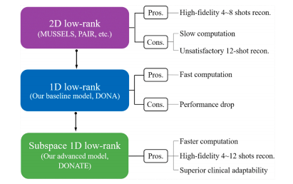
Fig. 1. Low-rank reconstruction for multi-shot DWI.
图1:多次激发弥散加权成像(DWI)的低秩重建
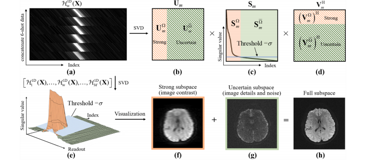
Fig. 2. Illustration of 1D low-rankness in the ms-iEPI DWI and visualization of strong and uncertain subspaces. (a) X is the k-space data of the 6-shot DWI. H 1 m D(X) is the lifted 1D Hankel matrix from the mth readout line of X, which is decomposed into (b) left signal subspace Um*, (c) singular values Sm, and (d) right signal subspace VH m with SVD. For each Hankel matrix, the signal subspace corresponding to singular values larger than the threshold σ is the strong subspace Ω, while the signal subspace corresponding to the singular values smaller than the threshold σ is the uncertain subspace Ω. (e) All singular values can be divided into strong and uncertain parts, and their corresponding subspaces and combined subspace are visualized in (f), (g), and (h), respectively. Note: × is the matrix multiplication
图2:多次激发交错回波平面成像(ms-iEPI)弥散加权成像(DWI)中一维低秩性的说明以及强子空间和不确定子空间的可视化。(a) X 是6次激发弥散加权成像的k空间数据。(\mathbf{H}{1mD}(\mathbf{X})) 是从 X 的第(m)条读出线提升得到的一维汉克尔矩阵,通过奇异值分解(SVD)将其分解为 (b) 左信号子空间 (\mathbf{U}{m})、(c) 奇异值 (\mathbf{S}{m}) 以及 (d) 右信号子空间 (\mathbf{V}{m}^{H})。对于每个汉克尔矩阵,对应奇异值大于阈值(\sigma)的信号子空间是强子空间(\Omega),而对应奇异值小于阈值(\sigma)的信号子空间是不确定子空间(\Omega)。(e) 所有奇异值可分为强部分和不确定部分,它们对应的子空间以及组合子空间分别在 (f)、(g) 和 (h) 中可视化显示。注意:× 表示矩阵乘法。
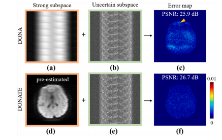
Fig. 3. A toy example of DONA and DONATE reconstruction. In DONA, (a) and (b) are the unreconstructed subspace, and (c) is the error map. In DONATE, (d) is the ground truth strong subspace, (e) is the unreconstructed uncertain subspace, and (f) is the error map. Note: The 6-shot 8-channel DWI data with noise (10 dB) are simulated as in (Qian et al., 2023b).
图3:DONA和DONATE重建的一个模拟示例。在DONA方法中,(a)和(b)是未重建的子空间,(c)是误差图。在DONATE方法中,(d)是真实的强子空间,(e)是未重建的不确定子空间,(f)是误差图。注意:如(钱等人,2023b)所述,模拟的是带有噪声(10分贝)的6次激发8通道弥散加权成像(DWI)数据。
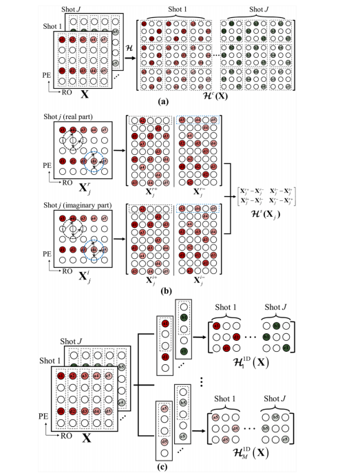
Fig. 4. The constructions of 2D block Hankel and 1D Hankel matrices. (a) and (b) are the 2D block Hankel matrices in MUSSELS and PAIR, respectively. (c) is the 1D Hankel matrix in DONA and DONATE. Note: X = [ X1, ..., Xj, ..., XJ ] is the multi-shot k-space data, and J is the shot number. The trajectory of the black sliding windows (circle) in (b) are from top to bottom and left to right, while the blue sliding windows (circle) in (b) are from bottom to top and right to left.
图4:二维分块汉克尔矩阵和一维汉克尔矩阵的构建。(a) 和 (b) 分别是MUSSELS和PAIR方法中的二维分块汉克尔矩阵。(c) 是DONA和DONATE方法中的一维汉克尔矩阵。注意:(\mathbf{X} = [ \mathbf{X}1, \ldots, \mathbf{X}j, \ldots, \mathbf{X}_J ]) 是多次激发的k空间数据,(J) 是激发次数。(b) 中黑色滑动窗口(圆圈)的轨迹是从上到下、从左到右,而 (b) 中的蓝色滑动窗口(圆圈)的轨迹是从下到上、从右到左。
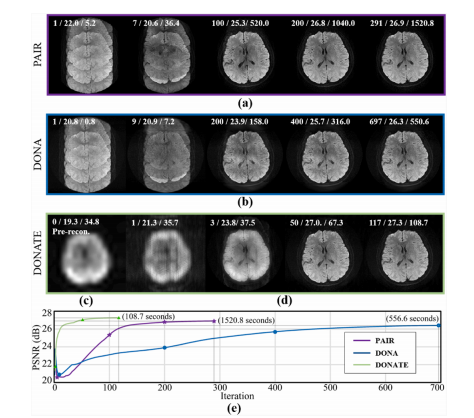
Fig. 5. Simulated 6-shot DWI reconstruction by PAIR, DONA, and DONATE. (a) and (b) are the reconstruction process of PAIR and DONA. (c) is a pre-estimated strong subspace in DONATE, and (d) is the recovery process of uncertain subspace in DONATE. (e) is the PSNR performance in iterations and final reconstruction (unit: seconds). Note: At the top of each image in (a)-(d), the Iteration / PSNR / Reconstruction time (unit: seconds) is given. The Phase encoding ×Readout is 256×256. The 8-channel DWI data with noise (10 dB) are simulated as in (Qian et al., 2023b). All methods are implemented with MATLAB and run on the same platform (Intel Core i9–9900X CPUs (128 GB RAM)) with the same stop criterion
图5:通过PAIR、DONA和DONATE方法对模拟的6次激发弥散加权成像(DWI)进行的重建。(a) 和 (b) 分别是PAIR和DONA的重建过程。(c) 是DONATE中预估计的强子空间,(d) 是DONATE中不确定子空间的恢复过程。(e) 是迭代过程中的峰值信噪比(PSNR)性能以及最终的重建情况(单位:秒)。注意:在(a)-(d) 中每张图像的顶部,给出了迭代次数 / 峰值信噪比 / 重建时间(单位:秒)。相位编码×读出的维度是256×256。如(钱等人,2023b)所述,模拟的是带有噪声(10分贝)的8通道弥散加权成像数据。所有方法均使用MATLAB实现,并在相同的平台(英特尔酷睿i9–9900X CPU(128GB内存))上运行,且采用相同的停止准则。
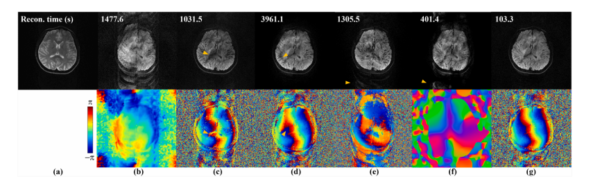
Fig. 6. Comparison study with 12-shot DWI data from DATASET I. (a) is the non-diffusion (b = 0) image. (b)-(g) are the results of MUSE, MUSSELS, PAIR, S-LORAKS, JULEP, and DONATE, respectively. The first row is magnitude images, and the second row is the shot phases. The reconstruction time (seconds) are given at the top of the image. Note: A fast version MUSSELS without conjugate symmetry is used.
图6:使用来自 数据集I 的12次激发弥散加权成像(DWI)数据进行的对比研究。(a) 是无弥散(b = 0)图像。(b)-(g) 分别是MUSE、MUSSELS、PAIR、S-LORAKS、JULEP和DONATE的结果。第一行是幅度图像,第二行是激发相位。图像顶部给出了重建时间(秒)。注意:使用的是无共轭对称性的快速版本MUSSELS。
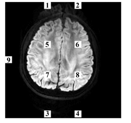
Fig. 7. Selected regions in ghost-to-signal ratio calculation. Each region has 9 ×9 voxels. Mean signal intensities in regions 1–4 are NIt, in regions 5–8 are SIt, and in region 9 is BI, where t = 1,2,3,4.
图7:在计算伪影与信号比率时所选的区域。每个区域有9×9个体素。区域1至4的平均信号强度为(NI_t),区域5至8的平均信号强度为(SI_t),区域9的平均信号强度为(BI),其中(t = 1,2,3,4)。
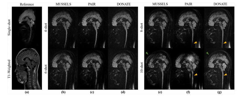
Fig. 8. Comparison study of ultra-high shot DWI on cervical spine from DATASET II. (a) are the distortion-free T1-weighted image (T1 W) acquired with fast spin echo sequence, and single-shot EPI DWI with severe distortion (resolution is 2.0 × 2.0 × 4.0 mm3 , and other parameters are the same as those of the multi-shot iEPI DWI). (b)-(g) are the reconstruction results of multi-shot iEPI DWI (from 4-shot to 10-shot). The artifacts in cervical spine and brain are marked with yellow and green arrows, respectively
图8:使用来自 数据集II 的超高激发次数颈椎弥散加权成像(DWI)进行的对比研究。(a) 是通过快速自旋回波序列采集的无畸变T1加权图像(T1 W),以及存在严重畸变的单次激发回波平面成像(EPI)弥散加权成像(分辨率为2.0×2.0×4.0立方毫米,其他参数与多次激发交错回波平面成像(iEPI)弥散加权成像相同)。(b)-(g) 是多次激发iEPI弥散加权成像(从4次激发到10次激发)的重建结果。颈椎和脑部的伪影分别用黄色和绿色箭头标出。
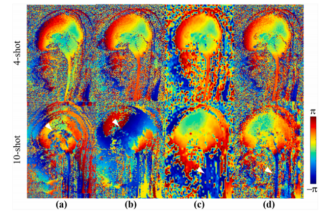
Fig. 9. Shot phase of 4-shot and 10-shot cervical spine DWI in Fig. 7. (a)-(d) are the MUSSELS, PAIR, pre-reconstruction, and final reconstruction of DONATE, respectively
图9:图7中4次激发和10次激发的颈椎弥散加权成像(DWI)的激发相位。(a)-(d) 分别是MUSSELS、PAIR、DONATE重建前以及DONATE最终重建的结果。
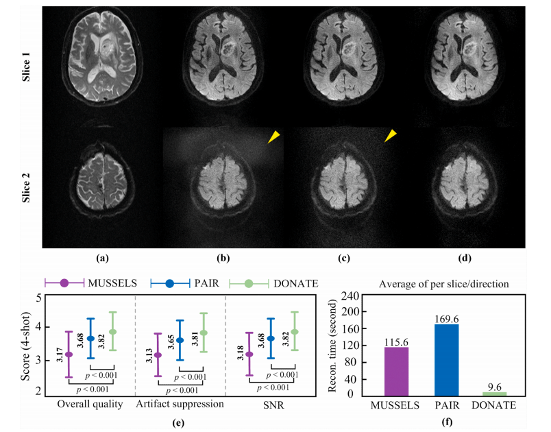
Fig. 10. Comparison and reader study with 4-shot patient DWI from DATASET III. (a) is the non-diffusion image (b-value=0). (b)-(d) are the reconstruction results by MUSSELS, PAIR, and DONATE, respectively. (e) are reader study scores on 60 slices that contain tumors or diseased regions from six patients. (f) is the reconstruction time. Note: The artifacts are marked by yellow arrows. Wilcoxon signed-rank test are used for scores analysis and p < 0.001 indicates statistically significant difference. All methods are implemented in MATLAB and run with 12 parallel computing cores on the same platform.
图10:使用来自数据集III的4次激发患者弥散加权成像(DWI)进行的对比和阅片者研究。(a) 是无弥散图像(b值 = 0)。(b)-(d) 分别是由MUSSELS、PAIR和DONATE得到的重建结果。(e) 是六位患者包含肿瘤或病变区域的60个切片的阅片者研究评分。(f) 是重建时间。注意:伪影用黄色箭头标出。使用威尔科克森符号秩检验进行评分分析,p < 0.001表示存在统计学显著差异。所有方法均在MATLAB中实现,并在同一平台上使用12个并行计算核心运行。
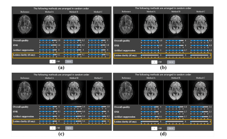
Fig. 11. Screenshots of the four radiologists’ scoring results for the third DWI image. (a)-(d) are the results of the 1st to 4th radiologists, respectively. Note: Reconstructed images by three methods are presented in random order on each radiologist’s screen.
图11:四位放射科医生对第三张弥散加权成像(DWI)图像的评分结果截图。(a)-(d) 分别是第一位到第四位放射科医生的评分结果。注意:三种方法重建的图像以随机顺序显示在每位放射科医生的屏幕上。
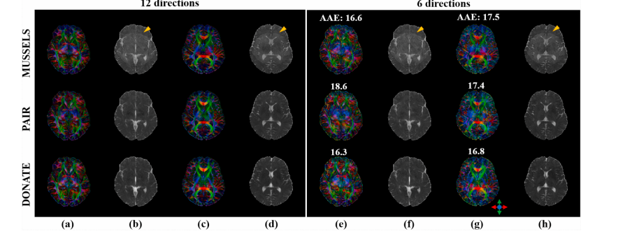
Fig. 12. Comparison study on 8-shot DTI data from DATASET VI. (a)(c) and (b)(d) are colored fractional anisotropy images (cFA) and mean diffusivity images (MD) estimated from all 12 diffusion directions, respectively. (e)(g) and (f)(h) are cFA and MD estimated from the 6 out of 12 diffusion directions, respectively. Average angular errors (AAE) are calculated with (a) and (c) as reference and marked in (e) and (g), respectively. AAEs are calculated for all 30 reconstructed cFA images (10 slices × 3 volunteers). Mean and standard deviation of AAE for MUSSELS, PAIR, and DONATE are 17.7 ± 1.64, 18.5 ± 1.80, and 17.4 ± 1.15, respectively. Note: MD and cFA are estimated by an open-source tool DIPY (Garyfallidis et al., 2014).
图12:使用来自数据集VI的8次激发弥散张量成像(DTI)数据进行的对比研究。(a)(c) 和 (b)(d) 分别是根据全部12个弥散方向估计得到的彩色各向异性分数图像(cFA)和平均弥散率图像(MD)。(e)(g) 和 (f)(h) 分别是根据12个弥散方向中的6个方向估计得到的cFA和MD。以(a) 和 (c) 作为参考计算平均角度误差(AAE),并分别标注在(e) 和 (g) 中。针对所有30张重建的cFA图像(10个切片×3位志愿者)计算AAE。MUSSELS、PAIR和DONATE的AAE的均值和标准差分别为17.7±1.64、18.5±1.80和17.4±1.15。注意:MD和cFA是通过开源工具DIPY(加里法利季斯等人,2014年)估计得到的。
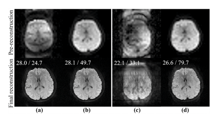
Fig. 13. Simulated noisy 4-shot and 8-shot DWI (10dB) reconstruction by DONATE with two different pre-reconstructions. (a) and (b) are 4-shot reconstruction with SENSE and PAIR as pre-reconstruction, respectively. (c) and (d) are the 8-shot reconstruction with SENSE and PAIR as pre-reconstruction, respectively. PSNR/reconstruction time (seconds) is marked at the top of the images.
图13:使用DONATE方法对模拟的含噪声(10分贝)的4次激发和8次激发弥散加权成像(DWI)进行重建,采用两种不同的预重建方式。(a) 和 (b) 分别是以SENSE和PAIR作为预重建的4次激发DWI的重建结果。(c) 和 (d) 分别是以SENSE和PAIR作为预重建的8次激发DWI的重建结果。峰值信噪比(PSNR)/重建时间(秒)标注在图像的顶部。
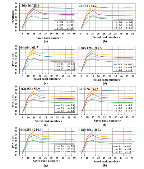
Fig. 14. DONATE reconstructions on the simulated noisy 4-shot 8-channel DWI data (10 dB) with different parameters, including k-space center size, σ, and r. Note: The Phase encoding × Readout is 256×256, The size of L1 × L2 / reconstruction time (unit: second) is marked on the top of each chart.
图14:使用DONATE方法对模拟的含噪声(10分贝)的4次激发8通道弥散加权成像(DWI)数据进行重建,采用不同的参数,包括k空间中心大小、(\sigma) 和 (r) 。注意:相位编码×读出维度为256×256。每个图表顶部标注了 (L_1×L_2) 的大小/重建时间(单位:秒)。
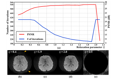
Fig. 15. The impact of η on reconstruction. (a) The number of iterations and PSNR performance. (b)-(e) are the reconstructed DWI image with η = 0.1, 1.9,2.0,2.1, respectively. Image artifacts are marked with yellow arrows. Note: Test is performed on a simulated noisy 6-shot 8-channel DWI (10 dB) data. Computation stops when the squared relative l2 norm of difference of reconstruction in two successive iterations is <1e-7. The allowed maximum number of iterations is 400.
图15:\(\eta\) 对重建的影响。(a) 迭代次数和峰值信噪比(PSNR)性能。(b)-(e) 分别是 \(\eta\) 取值为 0.1、1.9、2.0、2.1 时重建的弥散加权成像(DWI)图像。图像伪影用黄色箭头标出。注意:测试是在模拟的含噪声(10 分贝)的 6 次激发 8 通道弥散加权成像(DWI)数据上进行的。当两次连续迭代的重建结果的相对 \(l_2\) 范数平方小于 \(1\times10^{-7}\) 时计算停止。允许的最大迭代次数为 400 次。
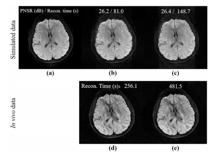
Fig. 16. Comparison of one-direction and two-direction DONATE with 8-shot simulated data (1st row) and in vivo data (2nd row). (a) is the noise-free ground truth. (b) and (d) are the results of one-direction DONATE, while (c) and (e) are the two-direction DONATE. PSNR and reconstruction time are marked at the top of the images. Note: The 1st row comes from a 8-channel simulated DWI data with noise (10 dB) as in (Qian et al., 2023b). The 2nd row comes from in vivo DATASET VI.
图16:使用8次激发的模拟数据(第一行)和体内数据(第二行)对单向DONATE和双向DONATE进行比较。(a) 是无噪声的真实数据。(b) 和 (d) 是单向DONATE的结果,而 (c) 和 (e) 是双向DONATE的结果。峰值信噪比(PSNR)和重建时间标注在图像的顶部。注意:第一行数据来自如(钱等人,2023b)所述的带有噪声(10分贝)的8通道模拟弥散加权成像(DWI)数据。第二行数据来自体内数据集VI。
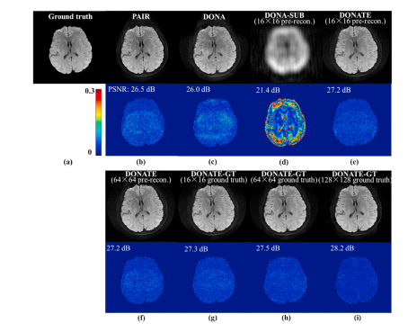
Fig. 17. Simulated 6-shot 8-channel DWI reconstruction with PAIR, DONA, DONA-SUB (not update strong subspace), DONATE, and DONATE-GT. (a) is the ground truth. (b) and (c) are the reconstructed image and error map of PAIR and DONA. (d) is the reconstructed image and error map of DONA-SUB. (e) and (f) are the reconstructed image and error map of DONATE, and the strong subspace is estimated from the pre-reconstructed 16×16, 64×64 k-space center. (g)-(i) are the reconstructed image and error map of DONATE-GT, and the strong subspace is estimated from the ground truth 16×16, 64×64, 128×128 kspace center, respectively. The computation time (seconds) of (b)-(i) are 1340.1, 370.7, 106.8, 81.2, 96.2, 22.8, 5.7, and 2.7, respectively.
图17:使用PAIR、DONA、DONA-SUB(不更新强子空间)、DONATE和DONATE-GT方法对模拟的6次激发8通道弥散加权成像(DWI)进行重建。(a) 是真实数据。(b) 和 (c) 分别是PAIR和DONA的重建图像和误差图。(d) 是DONA-SUB的重建图像和误差图。(e) 和 (f) 是DONATE的重建图像和误差图,强子空间是根据预重建的16×16、64×64的k空间中心估计得到的。(g)-(i) 是DONATE-GT的重建图像和误差图,强子空间分别是根据真实的16×16、64×64、128×128的k空间中心估计得到的。(b)-(i) 的计算时间(秒)分别为1340.1、370.7、106.8、81.2、96.2、22.8、5.7和2.7。
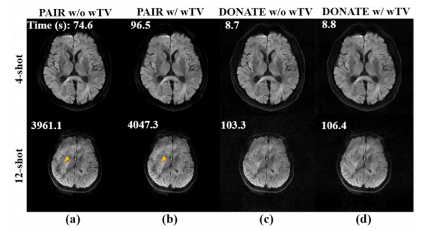
Fig. 18. Weighted total variation (wTV) study with in vivo 4-shot and 12-shot DWI reconstruction. (a)-(d) are the results of PAIR without wTV, PAIR with wTV, DONATE without wTV, and DONATE with wTV, respectively. The reconstruction time is marked at the top of each image.
图18:使用体内4次激发和12次激发弥散加权成像(DWI)重建进行的加权全变分(wTV)研究。(a)-(d) 分别是无加权全变分的PAIR方法、有加权全变分的PAIR方法、无加权全变分的DONATE方法和有加权全变分的DONATE方法的结果。每张图像的顶部都标注了重建时间。
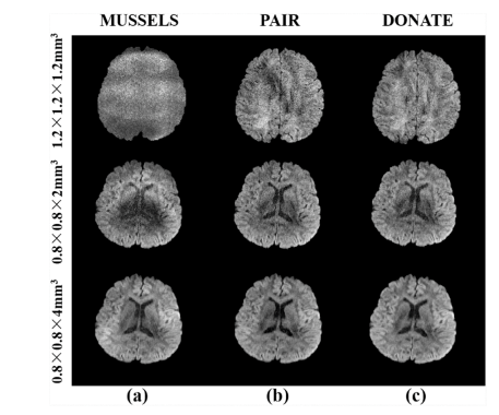
Fig. 19. Four-shot DWI images with 1.2 mm, 2 mm, and 4 mm slice thickness. Other imaging parameters are: in-plane resolution 1.2 × 1.2 mm2 for the 1st row, 0.8 × 0.8 mm2 for the 2nd and 3rd rows, 32 channels, b value 1000 s/ mm2 , and single average. All data are acquired with a 3.0 T Philips Ingenia CX scanner.
图19:切片厚度分别为1.2毫米、2毫米和4毫米的4次激发弥散加权成像(DWI)图像。其他成像参数为:第一行的面内分辨率为1.2×1.2平方毫米,第二行和第三行的面内分辨率为0.8×0.8平方毫米,32通道,b值为1000秒/平方毫米,且为单次平均。所有数据均使用3.0T飞利浦Ingenia CX扫描仪采集。
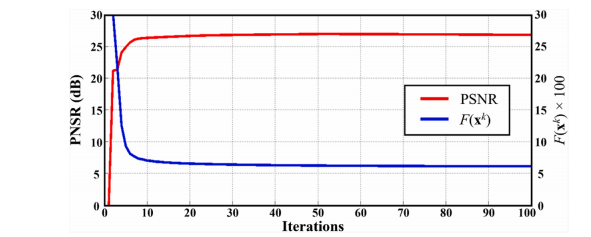
Fig. 20. Convergence curve of numerical algorithm of DONATE on a simulated noisy 6-shot 8-channel data (10 dB). Note: PSNR is measured when ground-truth is provided. When ground-truth is not available, F(xk ) = ‖ xk − xk− 1‖2/ ‖xk− 1‖2 measures the difference of reconstructed images between successive iterations.
图20:在模拟的含噪声(10分贝)的6次激发8通道数据上,DONATE数值算法的收敛曲线。注意:当有真实数据(参考数据)时测量峰值信噪比(PSNR)。当没有真实数据时,(F(\mathbf{x}k)=|\mathbf{x}k - \mathbf{x}{k - 1}|^2 / |\mathbf{x}{k - 1}|^2) 用于衡量连续迭代之间重建图像的差异。
Table
表
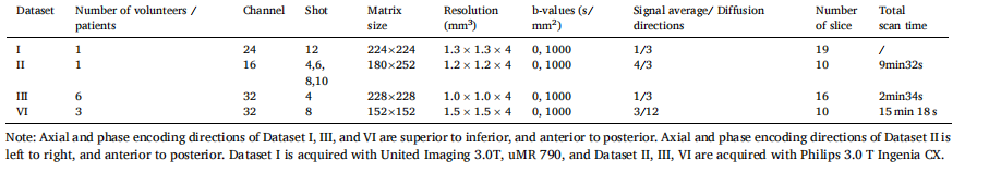
Table 1 Imaging parameters of four in vivo datasets in the comparison study.
表1 对比研究中四个体内数据集的成像参数。
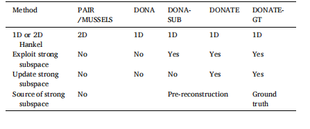
Table 2 Methods employed in ablation experiments.
表2 消融实验中所采用的方法。