Python----深度学习(基于深度学习Pytroch线性回归和曲线回归)
一、引言
在当今数据驱动的时代,深度学习已成为解决复杂问题的有力工具。它广泛应用于图像识别、自然语言处理和预测分析等领域。回归分析是统计学的一种基础方法,用于描述变量之间的关系。通过回归模型,我们可以预测连续的数值输出,这在经济学、工程学、医疗等领域有着至关重要的应用。
其中,线性回归是最简单且最常用的回归方法之一,它假设预测变量与目标变量之间存在线性关系。虽然线性回归在许多场景中表现良好,但当数据具有非线性特征时,它的预测能力可能会受到限制。在这些情况下,曲线回归(如多项式回归或其他非线性模型)通常可以提供更好的拟合效果。
二、线性回归
2.1、定义
线性回归是一种基本的预测分析方法,它通过拟合一条直线来描述自变量(特征)与因变量(目标)之间的关系。

2.2、设计思路
导入模块
import numpy as np
import torch
import random
import torch.nn as nn
import matplotlib.pyplot as plt
输入数据
point = [[1.8, 8.5], [1.6, 8.4], [2.3, 7.2], [0.7, 8.6], [1.8, 7.6], [4.9, 4.1], [2.5, 6.6], [4.4, 4.1],[7.4, 0.6], [1.9, 7.5],[5.8, 2.2], [6.8, 0.6], [2.9, 6.1], [5.6, 2.1], [1.0, 8.4], [5.3, 3.1], [3.2, 6.8], [3.2, 5.1],[6.4, 0.9], [2.9, 5.6],[5.5, 2.9], [4.7, 4.3], [8.0, 0.9], [2.1, 6.2], [7.2, 0.7], [4.1, 4.0], [5.6, 2.4], [1.3, 7.7],[3.2, 6.0], [4.7, 2.8],[5.4, 2.9], [4.0, 4.6], [4.3, 4.1], [1.3, 8.5], [2.5, 7.1], [4.1, 4.2], [5.4, 3.4], [6.4, 2.8],[7.0, 2.9], [2.4, 7.0],[1.2, 7.6], [7.5, 0.4], [7.7, 0.7], [1.8, 8.2], [0.6, 8.9], [4.5, 4.2], [7.3, 0.3], [7.4, 1.2],[4.0, 5.7], [7.0, 0.4],[6.7, 2.3], [1.3, 7.9], [1.7, 7.2], [4.8, 3.7], [1.3, 7.3], [5.4, 3.8], [3.9, 5.6], [3.1, 5.7],[3.2, 6.3], [2.5, 6.6],[0.9, 8.9], [1.4, 7.5], [0.8, 8.1], [1.9, 8.3], [4.2, 3.6], [1.7, 7.2], [7.7, 0.5], [5.5, 2.1],[4.2, 5.2], [3.9, 4.9],[4.2, 4.4], [4.0, 5.9], [4.3, 3.4], [7.0, 1.0], [7.6, 0.8], [7.3, 0.1], [5.6, 3.0], [6.4, 3.0],[-0.0, 9.1], [2.9, 6.7],[4.4, 3.6], [6.4, 2.2], [5.3, 3.2], [5.7, 2.7], [6.5, 1.5], [7.4, 1.1], [6.2, 2.1], [5.6, 1.4],[5.7, 2.0], [3.0, 5.2],[4.5, 5.6], [6.8, 1.7], [6.5, 1.3], [4.2, 4.5], [3.3, 6.5], [2.7, 5.2], [5.8, 3.5], [7.8, 0.9],[5.5, 3.0], [1.2, 8.0],[4.2, 4.2], [0.9, 8.6], [7.0, 1.0], [0.2, 9.6], [5.9, 3.0], [2.3, 6.5], [3.3, 5.1], [5.9, 2.2],[6.8, 1.7], [4.6, 3.8],[6.3, 1.3], [1.2, 8.4], [6.8, 1.6], [5.0, 2.3], [7.4, 0.1], [3.1, 5.9], [4.9, 3.8], [1.8, 7.5],[7.9, 0.3], [2.8, 5.2],[2.4, 7.2], [4.0, 4.0], [6.8, 1.7], [6.6, 1.9], [4.9, 4.4], [6.4, 2.9], [7.3, 0.7], [2.1, 7.6],[1.9, 7.7], [0.7, 9.2],[3.7, 4.8], [0.5, 8.9], [4.8, 4.4], [5.7, 2.7], [4.0, 3.8], [6.1, 1.6], [6.7, 0.3], [0.3, 8.5],[5.3, 1.7], [2.9, 5.6],[0.9, 7.8], [2.9, 6.5], [0.2, 8.8], [8.0, 0.7], [1.8, 6.7], [3.0, 6.0], [5.0, 3.7], [2.8, 5.3],[4.2, 5.2], [4.5, 5.2],[8.1, 0.6], [4.4, 3.9], [7.3, 1.4], [5.7, 2.0], [1.9, 7.2], [3.5, 4.4], [4.4, 4.4], [2.6, 6.3],[6.0, 2.9], [2.5, 7.1],[6.0, 2.3], [6.5, 1.2], [0.3, 9.6], [2.3, 6.6], [7.6, 0.4], [0.2, 9.3], [1.1, 8.7], [3.5, 5.2],[7.0, 2.0], [6.5, 2.1],[7.8, 0.6], [4.1, 4.3], [1.2, 8.9], [1.0, 8.9], [5.6, 3.4], [5.6, 2.0], [4.7, 3.3], [7.7, 0.8],[7.4, 1.4], [3.2, 4.9],[4.8, 3.9], [5.6, 2.8], [1.4, 8.7], [2.4, 7.2], [8.0, 0.3], [4.9, 3.8], [2.3, 6.9], [5.8, 2.7],[1.9, 7.0], [5.0, 2.9],[2.2, 7.4], [6.1, 2.6], [6.7, 1.0], [4.6, 3.6], [7.9, 0.2], [3.1, 5.8], [4.7, 4.1], [1.5, 8.1],[2.3, 7.0], [4.2, 5.0],[5.6, 2.2], [5.9, 2.6], [3.3, 4.8], [2.5, 5.6], [2.1, 7.5], [0.8, 7.4], [6.2, 2.6], [4.2, 3.8],[0.8, 8.3], [4.5, 4.1],[6.2, 2.0], [7.8, 1.0], [2.6, 6.0], [4.2, 4.2], [1.6, 7.8], [4.1, 4.2], [5.8, 2.7], [4.0, 5.8],[0.9, 7.8], [6.7, 1.6],[0.2, 8.2], [1.1, 7.7], [2.1, 7.1], [6.0, 2.8], [4.0, 4.9], [7.5, 1.6], [6.1, 1.7], [3.5, 5.9],[6.3, 1.6], [8.0, 0.3],[5.4, 2.6], [7.6, 0.2], [5.8, 2.9], [1.9, 6.6], [0.4, 8.2], [5.7, 2.1], [3.2, 6.2], [5.2, 3.5],[7.6, 0.2], [1.8, 7.3],[0.5, 8.4], [5.5, 3.6], [5.2, 3.4], [6.0, 2.3], [5.0, 3.8], [3.3, 5.5], [7.4, 1.3], [4.2, 4.3],[2.4, 7.0], [2.1, 6.5],[7.7, 0.7], [5.6, 2.7], [6.3, 1.4], [5.3, 2.0], [0.4, 8.5], [2.0, 7.7], [5.8, 3.8], [4.3, 4.5],[0.9, 8.9], [3.7, 4.7],[7.0, 1.5], [6.2, 2.0], [2.5, 6.2], [3.8, 5.5], [1.8, 8.4], [3.3, 5.5], [7.9, 0.4], [1.9, 7.8],[5.6, 3.1], [7.9, 0.6],[4.8, 3.7], [5.1, 3.9], [6.9, 1.3], [3.3, 5.8], [3.8, 5.1], [5.3, 3.5], [1.3, 7.8], [0.8, 8.2],[1.9, 7.8], [4.9, 3.6],[6.8, 2.4], [7.5, 0.2], [4.8, 3.3], [3.9, 4.4], [4.3, 4.2], [6.2, 1.9], [7.2, 0.8], [2.7, 6.0],[1.1, 7.7], [7.0, 0.1],[0.8, 7.3], [5.6, 3.5], [0.8, 8.1], [4.7, 3.8], [3.9, 4.5], [4.7, 3.2], [1.3, 7.7], [7.2, 0.8],[4.2, 4.0], [1.2, 8.9]]划分训练集和测试集
# 将 point1 分割为训练集和测试集
random.shuffle(point)  # 随机打乱数据
split_index = int(0.1 * len(point))  # 取前 10% 的数据作为测试集train_point = point[split_index:]
test_point = point[:split_index]x_train = np.array([point[0] for point in train_point])
y_train = np.array([point[1] for point in train_point])x_test = np.array([point[0] for point in test_point])
y_test = np.array([point[1] for point in test_point])
转换为Tensor张量
x_train = torch.from_numpy(x_train).float()
y_train = torch.from_numpy(y_train).float()
构建模型
class ModelClass(nn.Module):def __init__(self):super().__init__()self.layer1 = nn.Linear(1, 8)self.layer2 = nn.Linear(8, 1)def forward(self, x):x = torch.tanh(self.layer1(x))x = self.layer2(x)return xmodel = ModelClass()构建损失函数和优化器
criterion = nn.MSELoss()
optimizer = torch.optim.Adam(model.parameters(), lr=0.005, weight_decay=0.01)
模型训练
for n in range(1, 2001):# 前向传播y_pred = model(x_train.unsqueeze(1))# 计算损失loss = criterion(y_pred.squeeze(1), y_train)# 反向传播和优化optimizer.zero_grad()loss.backward()optimizer.step()if n % 100 == 0 or n == 1:print(n,loss.item())可视化
step_list = []
loss_list = []
test_step_list = []
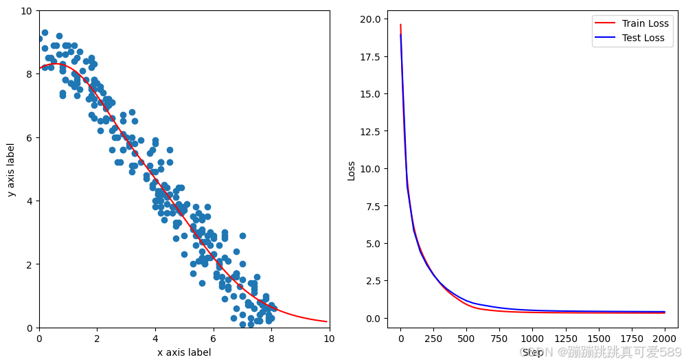
test_loss_list = []for n in range(1, 2001):# 前向传播y_pred = model(x_train.unsqueeze(1))# 计算损失loss = criterion(y_pred.squeeze(1), y_train)# 反向传播和优化optimizer.zero_grad()loss.backward()optimizer.step()# 更新右侧的损失图数据并绘制step_list.append(n)loss_list.append(loss.detach())# 显示频率设置if n % 100 == 0 or n == 1:print(n,loss.item())# 绘制左侧的拟合图ax1.clear()ax1.set_xlim(0, 10)ax1.set_ylim(0, 10)ax1.set_xlabel("x axis label")ax1.set_ylabel("y axis label")ax1.scatter(x_train, y_train)x_range = torch.tensor(np.arange(0, 10, 0.1)).unsqueeze(1).float()y_range = model(x_range).detach().numpy()ax1.plot(x_range, y_range, 'r') # 绘制拟合线# 计算测试集损失y_pred_test = model(torch.tensor(x_test).unsqueeze(1).float())loss_test = criterion(y_pred_test.squeeze(1), torch.from_numpy(y_test).float())test_step_list.append(n)test_loss_list.append(loss_test.detach())ax2.clear()ax2.plot(step_list, loss_list, 'r-', label='Train Loss')ax2.plot(test_step_list, test_loss_list, 'b-', label='Test Loss') # 绘制测试集损失ax2.set_xlabel("Step")ax2.set_ylabel("Loss")ax2.legend()
plt.show()完整代码
import numpy as np
import torch
import random
import torch.nn as nn
import matplotlib.pyplot as plt# 创造数据,数据集
point = [[1.8, 8.5], [1.6, 8.4], [2.3, 7.2], [0.7, 8.6], [1.8, 7.6], [4.9, 4.1], [2.5, 6.6], [4.4, 4.1],[7.4, 0.6], [1.9, 7.5],[5.8, 2.2], [6.8, 0.6], [2.9, 6.1], [5.6, 2.1], [1.0, 8.4], [5.3, 3.1], [3.2, 6.8], [3.2, 5.1],[6.4, 0.9], [2.9, 5.6],[5.5, 2.9], [4.7, 4.3], [8.0, 0.9], [2.1, 6.2], [7.2, 0.7], [4.1, 4.0], [5.6, 2.4], [1.3, 7.7],[3.2, 6.0], [4.7, 2.8],[5.4, 2.9], [4.0, 4.6], [4.3, 4.1], [1.3, 8.5], [2.5, 7.1], [4.1, 4.2], [5.4, 3.4], [6.4, 2.8],[7.0, 2.9], [2.4, 7.0],[1.2, 7.6], [7.5, 0.4], [7.7, 0.7], [1.8, 8.2], [0.6, 8.9], [4.5, 4.2], [7.3, 0.3], [7.4, 1.2],[4.0, 5.7], [7.0, 0.4],[6.7, 2.3], [1.3, 7.9], [1.7, 7.2], [4.8, 3.7], [1.3, 7.3], [5.4, 3.8], [3.9, 5.6], [3.1, 5.7],[3.2, 6.3], [2.5, 6.6],[0.9, 8.9], [1.4, 7.5], [0.8, 8.1], [1.9, 8.3], [4.2, 3.6], [1.7, 7.2], [7.7, 0.5], [5.5, 2.1],[4.2, 5.2], [3.9, 4.9],[4.2, 4.4], [4.0, 5.9], [4.3, 3.4], [7.0, 1.0], [7.6, 0.8], [7.3, 0.1], [5.6, 3.0], [6.4, 3.0],[-0.0, 9.1], [2.9, 6.7],[4.4, 3.6], [6.4, 2.2], [5.3, 3.2], [5.7, 2.7], [6.5, 1.5], [7.4, 1.1], [6.2, 2.1], [5.6, 1.4],[5.7, 2.0], [3.0, 5.2],[4.5, 5.6], [6.8, 1.7], [6.5, 1.3], [4.2, 4.5], [3.3, 6.5], [2.7, 5.2], [5.8, 3.5], [7.8, 0.9],[5.5, 3.0], [1.2, 8.0],[4.2, 4.2], [0.9, 8.6], [7.0, 1.0], [0.2, 9.6], [5.9, 3.0], [2.3, 6.5], [3.3, 5.1], [5.9, 2.2],[6.8, 1.7], [4.6, 3.8],[6.3, 1.3], [1.2, 8.4], [6.8, 1.6], [5.0, 2.3], [7.4, 0.1], [3.1, 5.9], [4.9, 3.8], [1.8, 7.5],[7.9, 0.3], [2.8, 5.2],[2.4, 7.2], [4.0, 4.0], [6.8, 1.7], [6.6, 1.9], [4.9, 4.4], [6.4, 2.9], [7.3, 0.7], [2.1, 7.6],[1.9, 7.7], [0.7, 9.2],[3.7, 4.8], [0.5, 8.9], [4.8, 4.4], [5.7, 2.7], [4.0, 3.8], [6.1, 1.6], [6.7, 0.3], [0.3, 8.5],[5.3, 1.7], [2.9, 5.6],[0.9, 7.8], [2.9, 6.5], [0.2, 8.8], [8.0, 0.7], [1.8, 6.7], [3.0, 6.0], [5.0, 3.7], [2.8, 5.3],[4.2, 5.2], [4.5, 5.2],[8.1, 0.6], [4.4, 3.9], [7.3, 1.4], [5.7, 2.0], [1.9, 7.2], [3.5, 4.4], [4.4, 4.4], [2.6, 6.3],[6.0, 2.9], [2.5, 7.1],[6.0, 2.3], [6.5, 1.2], [0.3, 9.6], [2.3, 6.6], [7.6, 0.4], [0.2, 9.3], [1.1, 8.7], [3.5, 5.2],[7.0, 2.0], [6.5, 2.1],[7.8, 0.6], [4.1, 4.3], [1.2, 8.9], [1.0, 8.9], [5.6, 3.4], [5.6, 2.0], [4.7, 3.3], [7.7, 0.8],[7.4, 1.4], [3.2, 4.9],[4.8, 3.9], [5.6, 2.8], [1.4, 8.7], [2.4, 7.2], [8.0, 0.3], [4.9, 3.8], [2.3, 6.9], [5.8, 2.7],[1.9, 7.0], [5.0, 2.9],[2.2, 7.4], [6.1, 2.6], [6.7, 1.0], [4.6, 3.6], [7.9, 0.2], [3.1, 5.8], [4.7, 4.1], [1.5, 8.1],[2.3, 7.0], [4.2, 5.0],[5.6, 2.2], [5.9, 2.6], [3.3, 4.8], [2.5, 5.6], [2.1, 7.5], [0.8, 7.4], [6.2, 2.6], [4.2, 3.8],[0.8, 8.3], [4.5, 4.1],[6.2, 2.0], [7.8, 1.0], [2.6, 6.0], [4.2, 4.2], [1.6, 7.8], [4.1, 4.2], [5.8, 2.7], [4.0, 5.8],[0.9, 7.8], [6.7, 1.6],[0.2, 8.2], [1.1, 7.7], [2.1, 7.1], [6.0, 2.8], [4.0, 4.9], [7.5, 1.6], [6.1, 1.7], [3.5, 5.9],[6.3, 1.6], [8.0, 0.3],[5.4, 2.6], [7.6, 0.2], [5.8, 2.9], [1.9, 6.6], [0.4, 8.2], [5.7, 2.1], [3.2, 6.2], [5.2, 3.5],[7.6, 0.2], [1.8, 7.3],[0.5, 8.4], [5.5, 3.6], [5.2, 3.4], [6.0, 2.3], [5.0, 3.8], [3.3, 5.5], [7.4, 1.3], [4.2, 4.3],[2.4, 7.0], [2.1, 6.5],[7.7, 0.7], [5.6, 2.7], [6.3, 1.4], [5.3, 2.0], [0.4, 8.5], [2.0, 7.7], [5.8, 3.8], [4.3, 4.5],[0.9, 8.9], [3.7, 4.7],[7.0, 1.5], [6.2, 2.0], [2.5, 6.2], [3.8, 5.5], [1.8, 8.4], [3.3, 5.5], [7.9, 0.4], [1.9, 7.8],[5.6, 3.1], [7.9, 0.6],[4.8, 3.7], [5.1, 3.9], [6.9, 1.3], [3.3, 5.8], [3.8, 5.1], [5.3, 3.5], [1.3, 7.8], [0.8, 8.2],[1.9, 7.8], [4.9, 3.6],[6.8, 2.4], [7.5, 0.2], [4.8, 3.3], [3.9, 4.4], [4.3, 4.2], [6.2, 1.9], [7.2, 0.8], [2.7, 6.0],[1.1, 7.7], [7.0, 0.1],[0.8, 7.3], [5.6, 3.5], [0.8, 8.1], [4.7, 3.8], [3.9, 4.5], [4.7, 3.2], [1.3, 7.7], [7.2, 0.8],[4.2, 4.0], [1.2, 8.9]]# 将 point1 分割为训练集和测试集
random.shuffle(point)  # 随机打乱数据
split_index = int(0.1 * len(point))  # 取前 10% 的数据作为测试集  # 划分数据集
train_point = point[split_index:]  # 训练集包含 90% 的数据
test_point = point[:split_index]    # 测试集为前 10% 的数据  # 将训练集和测试集的数据分别提取为特征和目标
x_train = np.array([point[0] for point in train_point])  # 训练特征
y_train = np.array([point[1] for point in train_point])  # 训练目标  x_test = np.array([point[0] for point in test_point])    # 测试特征
y_test = np.array([point[1] for point in test_point])    # 测试目标  # 转换为PyTorch的张量
x_train = torch.from_numpy(x_train).float()  # 将训练特征转换为浮点型张量
y_train = torch.from_numpy(y_train).float()  # 将训练目标转换为浮点型张量  # 定义前向模型
class ModelClass(nn.Module):  def __init__(self):  super().__init__()  # 定义网络层  self.layer1 = nn.Linear(1, 8)  # 第一个线性层,输入为1维,输出为8维  self.layer2 = nn.Linear(8, 1)   # 第二个线性层,输入为8维,输出为1维  def forward(self, x):  # 前向传播函数  x = torch.tanh(self.layer1(x))  # 第一个层的输出应用tanh激活函数  x = self.layer2(x)               # 经过第二个层  return x  # 实例化模型
model = ModelClass()  # 定义损失函数和优化器
criterion = nn.MSELoss()  # 均方误差损失函数
optimizer = torch.optim.Adam(model.parameters(), lr=0.005, weight_decay=0.01)  # Adam优化器  # 初始化绘图
fig, (ax1, ax2) = plt.subplots(1, 2, figsize=(12, 6))  # 创建绘图窗口,包含两个子图  # 开始迭代
step_list = []       # 用于存储训练的步骤
loss_list = []       # 用于存储训练损失
test_step_list = []  # 用于存储测试的步骤
test_loss_list = []  # 用于存储测试损失  for n in range(1, 2001):  # 训练迭代2000轮  # 前向传播  y_pred = model(x_train.unsqueeze(1))  # 将训练输入传入模型,reshape为合适维度  # 计算损失  loss = criterion(y_pred.squeeze(1), y_train)  # 计算模型预测值与真实值之间的损失  # 反向传播和优化  optimizer.zero_grad()  # 清除之前的梯度  loss.backward()        # 计算当前损失的梯度  optimizer.step()       # 更新模型参数  # 更新右侧的损失图数据并绘制  step_list.append(n)    # 记录当前步数  loss_list.append(loss.detach())  # 记录当前损失值  # 显示频率设置  if n % 100 == 0 or n == 1:  # 每100步输出一次损失值  print(n, loss.item())  # 打印当前步数和损失值  # 绘制左侧的拟合图  ax1.clear()  # 清除当前图  ax1.set_xlim(0, 10)  # 设置x轴范围  ax1.set_ylim(0, 10)  # 设置y轴范围  ax1.set_xlabel("x axis label")  # x轴标签  ax1.set_ylabel("y axis label")  # y轴标签  ax1.scatter(x_train, y_train)  # 绘制训练数据点  x_range = torch.tensor(np.arange(0, 10, 0.1)).unsqueeze(1).float()  # 生成预测输入范围  y_range = model(x_range).detach().numpy()  # 计算拟合线的预测输出  ax1.plot(x_range, y_range, 'r')  # 绘制拟合线  # 计算测试集损失  y_pred_test = model(torch.tensor(x_test).unsqueeze(1).float())  # 模型对测试集进行预测  loss_test = criterion(y_pred_test.squeeze(1), torch.from_numpy(y_test).float())  # 计算测试集损失  test_step_list.append(n)  # 记录测试步数  test_loss_list.append(loss_test.detach())  # 记录测试损失  ax2.clear()  # 清除当前测试损失图  ax2.plot(step_list, loss_list, 'r-', label='Train Loss')  # 绘制训练损失  ax2.plot(test_step_list, test_loss_list, 'b-', label='Test Loss')  # 绘制测试集损失  ax2.set_xlabel("Step")  # x轴标签  ax2.set_ylabel("Loss")  # y轴标签  ax2.legend()  # 显示图例  plt.show()  # 显示绘图窗口
三、曲线回归
3.1定义
曲线回归是一种用于拟合非线性关系的回归分析方法。与线性回归不同,曲线回归允许因变量与自变量之间存在更复杂的关系。常见的曲线回归形式包括多项式回归、指数回归和对数回归等。在多项式回归中,我们可以通过引入高次项来扩展模型的灵活性
常见模型
多项式回归:用于拟合二次或更高次的曲线,例如二次曲线
逻辑回归:虽然名字中有“回归”,逻辑回归实际上是用于分类问题的模型。
指数回归与对数回归:用于处理特定类型的数据关系,比如指数增长数据或对数增长数据。
3.2、设计思路
输入数据
point = [[0.5, 8.6], [0.5, 9.3], [0.6, 8.9], [0.6, 8.3], [0.6, 8.0], [0.7, 7.8], [0.7, 8.9], [0.7, 9.7],[0.7, 9.1], [0.8, 9.2],[0.8, 8.5], [0.8, 8.4], [0.9, 8.8], [0.9, 8.6], [0.9, 8.2], [1.0, 8.2], [1.0, 6.6], [1.0, 6.3],[1.0, 6.9], [1.1, 7.1],[1.1, 7.7], [1.1, 6.5], [1.2, 7.0], [1.2, 7.7], [1.2, 6.1], [1.3, 7.7], [1.3, 6.5], [1.3, 6.9],[1.3, 5.3], [1.4, 5.7],[1.4, 5.8], [1.4, 5.6], [1.5, 6.8], [1.5, 6.7], [1.5, 6.6], [1.6, 3.6], [1.6, 5.3], [1.6, 6.9],[1.6, 5.9], [1.7, 6.0],[1.7, 4.7], [1.7, 5.0], [1.8, 4.5], [1.8, 5.6], [1.8, 4.2], [1.9, 3.8], [1.9, 4.5], [1.9, 5.8],[1.9, 6.7], [2.0, 6.5],[2.0, 6.3], [2.0, 4.9], [2.1, 5.9], [2.1, 3.6], [2.1, 3.8], [2.2, 4.8], [2.2, 4.3], [2.2, 4.6],[2.2, 4.1], [2.3, 3.5],[2.3, 2.9], [2.3, 4.4], [2.4, 4.5], [2.4, 3.6], [2.4, 4.3], [2.5, 5.0], [2.5, 2.3], [2.5, 4.4],[2.5, 6.0], [2.6, 3.4],[2.6, 3.6], [2.6, 3.6], [2.7, 4.9], [2.7, 3.6], [2.7, 5.1], [2.8, 5.1], [2.8, 3.5], [2.8, 2.0],[2.8, 3.7], [2.9, 2.5],[2.9, 3.3], [2.9, 2.8], [3.0, 2.5], [3.0, 1.4], [3.0, 4.1], [3.1, 2.8], [3.1, 4.1], [3.1, 2.2],[3.1, 3.1], [3.2, 3.2],[3.2, 3.0], [3.2, 3.7], [3.3, 3.7], [3.3, 2.9], [3.3, 4.0], [3.4, 2.7], [3.4, 3.0], [3.4, 2.3],[3.4, 1.8], [3.5, 3.4],[3.5, 3.9], [3.5, 3.1], [3.6, 3.1], [3.6, 2.4], [3.6, 2.1], [3.7, 2.3], [3.7, 1.3], [3.7, 2.7],[3.8, 2.0], [3.8, 2.2],[3.8, 3.0], [3.8, 2.0], [3.9, 3.1], [3.9, 1.9], [3.9, 0.0], [4.0, 1.6], [4.0, 1.9], [4.0, 1.8],[4.1, 2.6], [4.1, 2.0],[4.1, 1.2], [4.1, 2.5], [4.2, 2.0], [4.2, 0.1], [4.2, 1.7], [4.3, 1.2], [4.3, 2.4], [4.3, 2.1],[4.4, 1.3], [4.4, 1.0],[4.4, 1.6], [4.4, 2.8], [4.5, 2.8], [4.5, 2.1], [4.5, 1.9], [4.6, 3.0], [4.6, 2.3], [4.6, 2.3],[4.7, 3.0], [4.7, 0.4],[4.7, 1.6], [4.7, 1.1], [4.8, 2.6], [4.8, 2.9], [4.8, 2.9], [4.9, 2.5], [4.9, 2.4], [4.9, 1.9],[5.0, 1.9], [5.0, 2.9],[5.0, 1.4], [5.0, 2.0], [5.1, 3.4], [5.1, 2.5], [5.1, 1.7], [5.2, 2.7], [5.2, 2.2], [5.2, 1.9],[5.3, 1.5], [5.3, 2.6],[5.3, 1.9], [5.3, 1.2], [5.4, 2.2], [5.4, 2.6], [5.4, 1.2], [5.5, 1.8], [5.5, 2.4], [5.5, 3.0],[5.6, 2.7], [5.6, 3.6],[5.6, 2.2], [5.6, 2.4], [5.7, 2.2], [5.7, 3.3], [5.7, 2.2], [5.8, 3.0], [5.8, 0.9], [5.8, 2.6],[5.9, 2.5], [5.9, 1.5],[5.9, 2.4], [5.9, 2.1], [6.0, 2.2], [6.0, 1.7], [6.0, 2.8], [6.1, 1.4], [6.1, 2.5], [6.1, 2.0],[6.2, 2.5], [6.2, 2.5],[6.2, 1.0], [6.2, 2.4], [6.3, 1.1], [6.3, 2.9], [6.3, 3.5], [6.4, 2.3], [6.4, 5.0], [6.4, 2.8],[6.5, 1.5], [6.5, 4.0],[6.5, 3.6], [6.6, 3.8], [6.6, 2.7], [6.6, 2.6], [6.6, 2.1], [6.7, 3.1], [6.7, 3.6], [6.7, 3.5],[6.8, 2.7], [6.8, 3.0],[6.8, 2.5], [6.9, 2.9], [6.9, 3.9], [6.9, 3.6], [6.9, 3.4], [7.0, 3.4], [7.0, 3.4], [7.0, 4.5],[7.1, 3.9], [7.1, 4.6],[7.1, 4.4], [7.2, 4.1], [7.2, 3.2], [7.2, 2.7], [7.2, 4.2], [7.3, 4.1], [7.3, 5.7], [7.3, 3.7],[7.4, 3.0], [7.4, 4.0],[7.4, 3.9], [7.5, 4.3], [7.5, 3.5], [7.5, 4.4], [7.5, 6.2], [7.6, 4.0], [7.6, 5.7], [7.6, 6.6],[7.7, 6.1], [7.7, 5.4],[7.7, 2.5], [7.8, 5.6], [7.8, 4.1], [7.8, 5.9], [7.8, 5.1], [7.9, 4.5], [7.9, 5.1], [7.9, 5.5],[8.0, 5.8], [8.0, 5.0],[8.0, 6.0], [8.1, 5.8], [8.1, 5.9], [8.1, 5.6], [8.1, 5.2], [8.2, 4.0], [8.2, 6.4], [8.2, 4.5],[8.3, 6.2], [8.3, 5.7],[8.3, 5.3], [8.4, 4.9], [8.4, 6.9], [8.4, 5.0], [8.4, 7.4], [8.5, 5.0], [8.5, 7.5], [8.5, 7.1],[8.6, 6.4], [8.6, 6.0],[8.6, 7.5], [8.7, 5.8], [8.7, 7.7], [8.7, 6.2], [8.7, 6.6], [8.8, 6.2], [8.8, 8.1], [8.8, 7.7],[8.9, 7.4], [8.9, 8.2],[8.9, 7.4], [9.0, 7.6], [9.0, 6.7], [9.0, 7.7], [9.0, 8.2], [9.1, 7.7], [9.1, 9.2], [9.1, 9.1],[9.2, 8.5], [9.2, 7.4],[9.2, 8.5], [9.3, 9.2], [9.3, 8.3], [9.3, 9.7], [9.3, 8.5], [9.4, 8.2], [9.4, 9.9], [9.4, 8.5],[9.5, 9.9], [9.5, 8.7]]划分训练集和测试集
# 将 point1 分割为训练集和测试集
random.shuffle(point)  # 随机打乱数据
split_index = int(0.1 * len(point))  # 取前 10% 的数据作为测试集train_point = point[split_index:]
test_point = point[:split_index]x_train = np.array([point[0] for point in train_point])
y_train = np.array([point[1] for point in train_point])x_test = np.array([point[0] for point in test_point])
y_test = np.array([point[1] for point in test_point])
转换为Tensor张量
x_train = torch.from_numpy(x_train).float()
y_train = torch.from_numpy(y_train).float()
构建模型
class ModelClass(nn.Module):def __init__(self):super().__init__()self.layer1 = nn.Linear(1, 8)self.layer2 = nn.Linear(8, 1)def forward(self, x):x = torch.tanh(self.layer1(x))x = self.layer2(x)return xmodel = ModelClass()构建损失函数和优化器
criterion = nn.MSELoss()
optimizer = torch.optim.Adam(model.parameters(), lr=0.005, weight_decay=0.01)
模型训练
for n in range(1, 2001):# 前向传播y_pred = model(x_train.unsqueeze(1))# 计算损失loss = criterion(y_pred.squeeze(1), y_train)# 反向传播和优化optimizer.zero_grad()loss.backward()optimizer.step()if n % 100 == 0 or n == 1:print(n,loss.item())可视化
step_list = []
loss_list = []
test_step_list = []
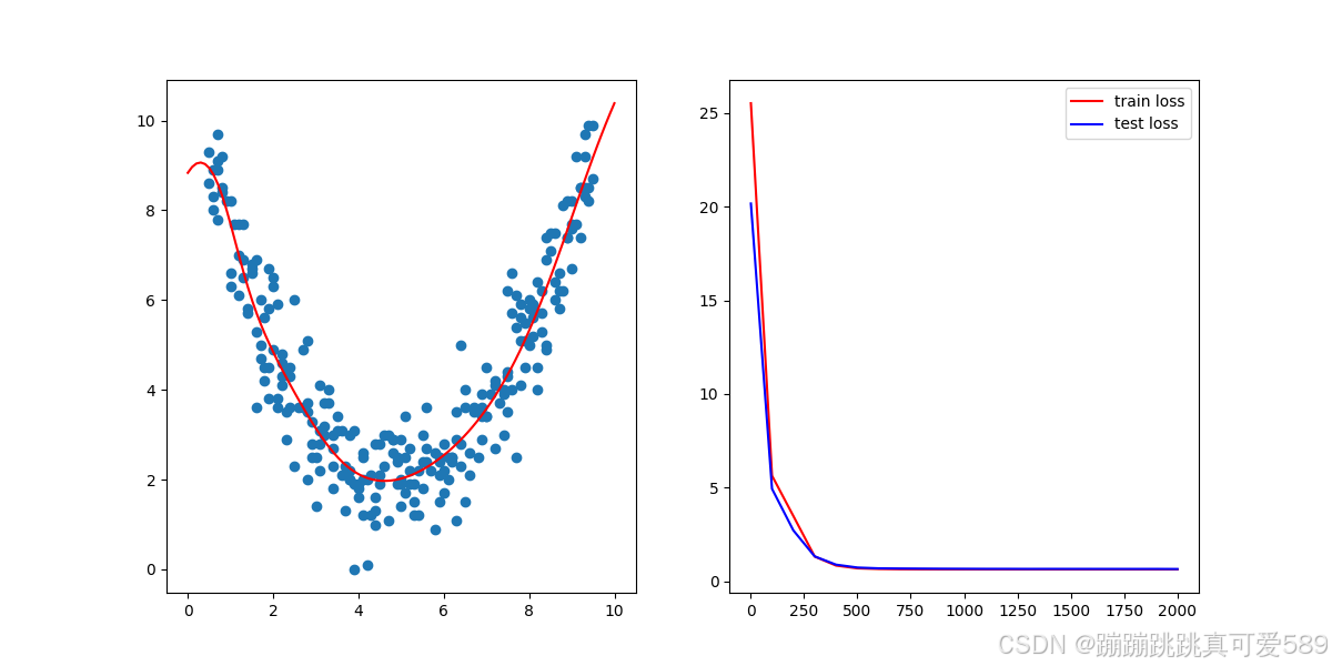
test_loss_list = []for n in range(1, 2001):# 前向传播y_pred = model(x_train.unsqueeze(1))# 计算损失loss = criterion(y_pred.squeeze(1), y_train)# 反向传播和优化optimizer.zero_grad()loss.backward()optimizer.step()# 更新右侧的损失图数据并绘制step_list.append(n)loss_list.append(loss.detach())# 显示频率设置if n % 100 == 0 or n == 1:print(n,loss.item())# 绘制左侧的拟合图ax1.clear()ax1.set_xlim(0, 10)ax1.set_ylim(0, 10)ax1.set_xlabel("x axis label")ax1.set_ylabel("y axis label")ax1.scatter(x_train, y_train)x_range = torch.tensor(np.arange(0, 10, 0.1)).unsqueeze(1).float()y_range = model(x_range).detach().numpy()ax1.plot(x_range, y_range, 'r') # 绘制拟合线# 计算测试集损失y_pred_test = model(torch.tensor(x_test).unsqueeze(1).float())loss_test = criterion(y_pred_test.squeeze(1), torch.from_numpy(y_test).float())test_step_list.append(n)test_loss_list.append(loss_test.detach())ax2.clear()ax2.plot(step_list, loss_list, 'r-', label='Train Loss')ax2.plot(test_step_list, test_loss_list, 'b-', label='Test Loss') # 绘制测试集损失ax2.set_xlabel("Step")ax2.set_ylabel("Loss")ax2.legend()
plt.show()完整代码
import numpy as np
import torch
import random
import torch.nn as nn
import matplotlib.pyplot as plt# 创造数据,数据集
point = [[0.5, 8.6], [0.5, 9.3], [0.6, 8.9], [0.6, 8.3], [0.6, 8.0], [0.7, 7.8], [0.7, 8.9], [0.7, 9.7],[0.7, 9.1], [0.8, 9.2],[0.8, 8.5], [0.8, 8.4], [0.9, 8.8], [0.9, 8.6], [0.9, 8.2], [1.0, 8.2], [1.0, 6.6], [1.0, 6.3],[1.0, 6.9], [1.1, 7.1],[1.1, 7.7], [1.1, 6.5], [1.2, 7.0], [1.2, 7.7], [1.2, 6.1], [1.3, 7.7], [1.3, 6.5], [1.3, 6.9],[1.3, 5.3], [1.4, 5.7],[1.4, 5.8], [1.4, 5.6], [1.5, 6.8], [1.5, 6.7], [1.5, 6.6], [1.6, 3.6], [1.6, 5.3], [1.6, 6.9],[1.6, 5.9], [1.7, 6.0],[1.7, 4.7], [1.7, 5.0], [1.8, 4.5], [1.8, 5.6], [1.8, 4.2], [1.9, 3.8], [1.9, 4.5], [1.9, 5.8],[1.9, 6.7], [2.0, 6.5],[2.0, 6.3], [2.0, 4.9], [2.1, 5.9], [2.1, 3.6], [2.1, 3.8], [2.2, 4.8], [2.2, 4.3], [2.2, 4.6],[2.2, 4.1], [2.3, 3.5],[2.3, 2.9], [2.3, 4.4], [2.4, 4.5], [2.4, 3.6], [2.4, 4.3], [2.5, 5.0], [2.5, 2.3], [2.5, 4.4],[2.5, 6.0], [2.6, 3.4],[2.6, 3.6], [2.6, 3.6], [2.7, 4.9], [2.7, 3.6], [2.7, 5.1], [2.8, 5.1], [2.8, 3.5], [2.8, 2.0],[2.8, 3.7], [2.9, 2.5],[2.9, 3.3], [2.9, 2.8], [3.0, 2.5], [3.0, 1.4], [3.0, 4.1], [3.1, 2.8], [3.1, 4.1], [3.1, 2.2],[3.1, 3.1], [3.2, 3.2],[3.2, 3.0], [3.2, 3.7], [3.3, 3.7], [3.3, 2.9], [3.3, 4.0], [3.4, 2.7], [3.4, 3.0], [3.4, 2.3],[3.4, 1.8], [3.5, 3.4],[3.5, 3.9], [3.5, 3.1], [3.6, 3.1], [3.6, 2.4], [3.6, 2.1], [3.7, 2.3], [3.7, 1.3], [3.7, 2.7],[3.8, 2.0], [3.8, 2.2],[3.8, 3.0], [3.8, 2.0], [3.9, 3.1], [3.9, 1.9], [3.9, 0.0], [4.0, 1.6], [4.0, 1.9], [4.0, 1.8],[4.1, 2.6], [4.1, 2.0],[4.1, 1.2], [4.1, 2.5], [4.2, 2.0], [4.2, 0.1], [4.2, 1.7], [4.3, 1.2], [4.3, 2.4], [4.3, 2.1],[4.4, 1.3], [4.4, 1.0],[4.4, 1.6], [4.4, 2.8], [4.5, 2.8], [4.5, 2.1], [4.5, 1.9], [4.6, 3.0], [4.6, 2.3], [4.6, 2.3],[4.7, 3.0], [4.7, 0.4],[4.7, 1.6], [4.7, 1.1], [4.8, 2.6], [4.8, 2.9], [4.8, 2.9], [4.9, 2.5], [4.9, 2.4], [4.9, 1.9],[5.0, 1.9], [5.0, 2.9],[5.0, 1.4], [5.0, 2.0], [5.1, 3.4], [5.1, 2.5], [5.1, 1.7], [5.2, 2.7], [5.2, 2.2], [5.2, 1.9],[5.3, 1.5], [5.3, 2.6],[5.3, 1.9], [5.3, 1.2], [5.4, 2.2], [5.4, 2.6], [5.4, 1.2], [5.5, 1.8], [5.5, 2.4], [5.5, 3.0],[5.6, 2.7], [5.6, 3.6],[5.6, 2.2], [5.6, 2.4], [5.7, 2.2], [5.7, 3.3], [5.7, 2.2], [5.8, 3.0], [5.8, 0.9], [5.8, 2.6],[5.9, 2.5], [5.9, 1.5],[5.9, 2.4], [5.9, 2.1], [6.0, 2.2], [6.0, 1.7], [6.0, 2.8], [6.1, 1.4], [6.1, 2.5], [6.1, 2.0],[6.2, 2.5], [6.2, 2.5],[6.2, 1.0], [6.2, 2.4], [6.3, 1.1], [6.3, 2.9], [6.3, 3.5], [6.4, 2.3], [6.4, 5.0], [6.4, 2.8],[6.5, 1.5], [6.5, 4.0],[6.5, 3.6], [6.6, 3.8], [6.6, 2.7], [6.6, 2.6], [6.6, 2.1], [6.7, 3.1], [6.7, 3.6], [6.7, 3.5],[6.8, 2.7], [6.8, 3.0],[6.8, 2.5], [6.9, 2.9], [6.9, 3.9], [6.9, 3.6], [6.9, 3.4], [7.0, 3.4], [7.0, 3.4], [7.0, 4.5],[7.1, 3.9], [7.1, 4.6],[7.1, 4.4], [7.2, 4.1], [7.2, 3.2], [7.2, 2.7], [7.2, 4.2], [7.3, 4.1], [7.3, 5.7], [7.3, 3.7],[7.4, 3.0], [7.4, 4.0],[7.4, 3.9], [7.5, 4.3], [7.5, 3.5], [7.5, 4.4], [7.5, 6.2], [7.6, 4.0], [7.6, 5.7], [7.6, 6.6],[7.7, 6.1], [7.7, 5.4],[7.7, 2.5], [7.8, 5.6], [7.8, 4.1], [7.8, 5.9], [7.8, 5.1], [7.9, 4.5], [7.9, 5.1], [7.9, 5.5],[8.0, 5.8], [8.0, 5.0],[8.0, 6.0], [8.1, 5.8], [8.1, 5.9], [8.1, 5.6], [8.1, 5.2], [8.2, 4.0], [8.2, 6.4], [8.2, 4.5],[8.3, 6.2], [8.3, 5.7],[8.3, 5.3], [8.4, 4.9], [8.4, 6.9], [8.4, 5.0], [8.4, 7.4], [8.5, 5.0], [8.5, 7.5], [8.5, 7.1],[8.6, 6.4], [8.6, 6.0],[8.6, 7.5], [8.7, 5.8], [8.7, 7.7], [8.7, 6.2], [8.7, 6.6], [8.8, 6.2], [8.8, 8.1], [8.8, 7.7],[8.9, 7.4], [8.9, 8.2],[8.9, 7.4], [9.0, 7.6], [9.0, 6.7], [9.0, 7.7], [9.0, 8.2], [9.1, 7.7], [9.1, 9.2], [9.1, 9.1],[9.2, 8.5], [9.2, 7.4],[9.2, 8.5], [9.3, 9.2], [9.3, 8.3], [9.3, 9.7], [9.3, 8.5], [9.4, 8.2], [9.4, 9.9], [9.4, 8.5],[9.5, 9.9], [9.5, 8.7]]# 将 point1 分割为训练集和测试集
random.shuffle(point)  # 随机打乱数据
split_index = int(0.1 * len(point))  # 取前 10% 的数据作为测试集  # 划分数据集
train_point = point[split_index:]  # 训练集包含 90% 的数据
test_point = point[:split_index]    # 测试集为前 10% 的数据  # 将训练集和测试集的数据分别提取为特征和目标
x_train = np.array([point[0] for point in train_point])  # 训练特征
y_train = np.array([point[1] for point in train_point])  # 训练目标  x_test = np.array([point[0] for point in test_point])    # 测试特征
y_test = np.array([point[1] for point in test_point])    # 测试目标  # 转换为PyTorch的张量
x_train = torch.from_numpy(x_train).float()  # 将训练特征转换为浮点型张量
y_train = torch.from_numpy(y_train).float()  # 将训练目标转换为浮点型张量  # 定义前向模型
class ModelClass(nn.Module):  def __init__(self):  super().__init__()  # 定义网络层  self.layer1 = nn.Linear(1, 8)  # 第一个线性层,输入为1维,输出为8维  self.layer2 = nn.Linear(8, 1)   # 第二个线性层,输入为8维,输出为1维  def forward(self, x):  # 前向传播函数  x = torch.tanh(self.layer1(x))  # 第一个层的输出应用tanh激活函数  x = self.layer2(x)               # 经过第二个层  return x  # 实例化模型
model = ModelClass()  # 定义损失函数和优化器
criterion = nn.MSELoss()  # 均方误差损失函数
optimizer = torch.optim.Adam(model.parameters(), lr=0.005, weight_decay=0.01)  # Adam优化器  # 初始化绘图
fig, (ax1, ax2) = plt.subplots(1, 2, figsize=(12, 6))  # 创建绘图窗口,包含两个子图  # 开始迭代
step_list = []       # 用于存储训练的步骤
loss_list = []       # 用于存储训练损失
test_step_list = []  # 用于存储测试的步骤
test_loss_list = []  # 用于存储测试损失  for n in range(1, 2001):  # 训练迭代2000轮  # 前向传播  y_pred = model(x_train.unsqueeze(1))  # 将训练输入传入模型,reshape为合适维度  # 计算损失  loss = criterion(y_pred.squeeze(1), y_train)  # 计算模型预测值与真实值之间的损失  # 反向传播和优化  optimizer.zero_grad()  # 清除之前的梯度  loss.backward()        # 计算当前损失的梯度  optimizer.step()       # 更新模型参数  # 更新右侧的损失图数据并绘制  step_list.append(n)    # 记录当前步数  loss_list.append(loss.detach())  # 记录当前损失值  # 显示频率设置  if n % 100 == 0 or n == 1:  # 每100步输出一次损失值  print(n, loss.item())  # 打印当前步数和损失值  # 绘制左侧的拟合图  ax1.clear()  # 清除当前图  ax1.set_xlim(0, 10)  # 设置x轴范围  ax1.set_ylim(0, 10)  # 设置y轴范围  ax1.set_xlabel("x axis label")  # x轴标签  ax1.set_ylabel("y axis label")  # y轴标签  ax1.scatter(x_train, y_train)  # 绘制训练数据点  x_range = torch.tensor(np.arange(0, 10, 0.1)).unsqueeze(1).float()  # 生成预测输入范围  y_range = model(x_range).detach().numpy()  # 计算拟合线的预测输出  ax1.plot(x_range, y_range, 'r')  # 绘制拟合线  # 计算测试集损失  y_pred_test = model(torch.tensor(x_test).unsqueeze(1).float())  # 模型对测试集进行预测  loss_test = criterion(y_pred_test.squeeze(1), torch.from_numpy(y_test).float())  # 计算测试集损失  test_step_list.append(n)  # 记录测试步数  test_loss_list.append(loss_test.detach())  # 记录测试损失  ax2.clear()  # 清除当前测试损失图  ax2.plot(step_list, loss_list, 'r-', label='Train Loss')  # 绘制训练损失  ax2.plot(test_step_list, test_loss_list, 'b-', label='Test Loss')  # 绘制测试集损失  ax2.set_xlabel("Step")  # x轴标签  ax2.set_ylabel("Loss")  # y轴标签  ax2.legend()  # 显示图例  plt.show()  # 显示绘图窗口