Python----深度学习（神经网络的过拟合解决方案）

一、正则化

1.1、正则化

        正则化是一种用于控制模型复杂度的技术。它通过在损失函数中添加额外的项（正则 化项）来降低模型的复杂度，以防止过拟合。

        在机器学习中，模型的目标是在训练数据上获得较好的拟合效果。然而，过于复杂的 模型可能会在训练数据上表现良好，但在未见过的数据上表现较差，这种现象称为过 拟合。为了避免过拟合，正则化技术被引入。

1.2、为什么加入正则化可以解决过拟合？

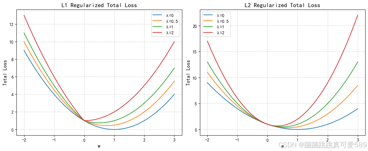
        加入正则化之后，想要损失函数尽可能的小，不仅仅要让原来的MSE的 值尽可能的小，还需要让后面正则化项的值尽可能的小。 要让正则化项的的值尽可能的小，那么就要使的参数 尽可能的小。

        参数 小和解决过拟合的关系：

                过拟合的实质是模型过于复杂或者训练样本较少，也可以理解为：针对当前 样本，模型过于复杂。 模型的复杂程度是由参数的个数和参数大小范围决定的，那么如果降低参数 的大 小范围，就可以降低模型的复杂度，因此可以用来解决过拟合问题。

1.3、正则化的基本思想

        正则化的基本思想是在损失函数中引入一个额外的项，该项与模型的复杂度相关。这 个额外的项可以是参数的平方和（L2正则化），参数的绝对值和（L1正则化）或其 他形式的复杂度度量。通过调整正则化参数，可以控制正则化项在损失函数中的权 重。

        正则化的目的是通过在损失函数中添加一个正则项（通常是权重的 L1 或 L2 范 数），以惩罚模型的复杂度，从而避免过拟合问题。

1.4、L1正则化和L2正则化

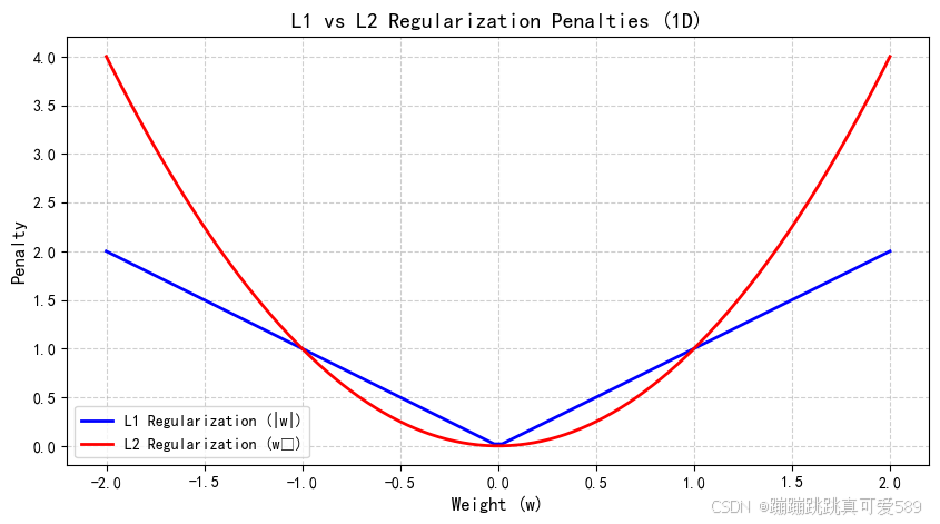
特性	L1正则化	L2正则化
稀疏性	产生稀疏解（部分权重为零）	不产生稀疏解（权重接近零）
优化特性	在零点不可导，需特殊处理	在零点可导，优化稳定
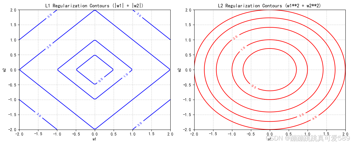
几何形状（2D）	菱形	圆形
应用场景	特征选择、高维稀疏数据	防止过拟合、平滑权重分布

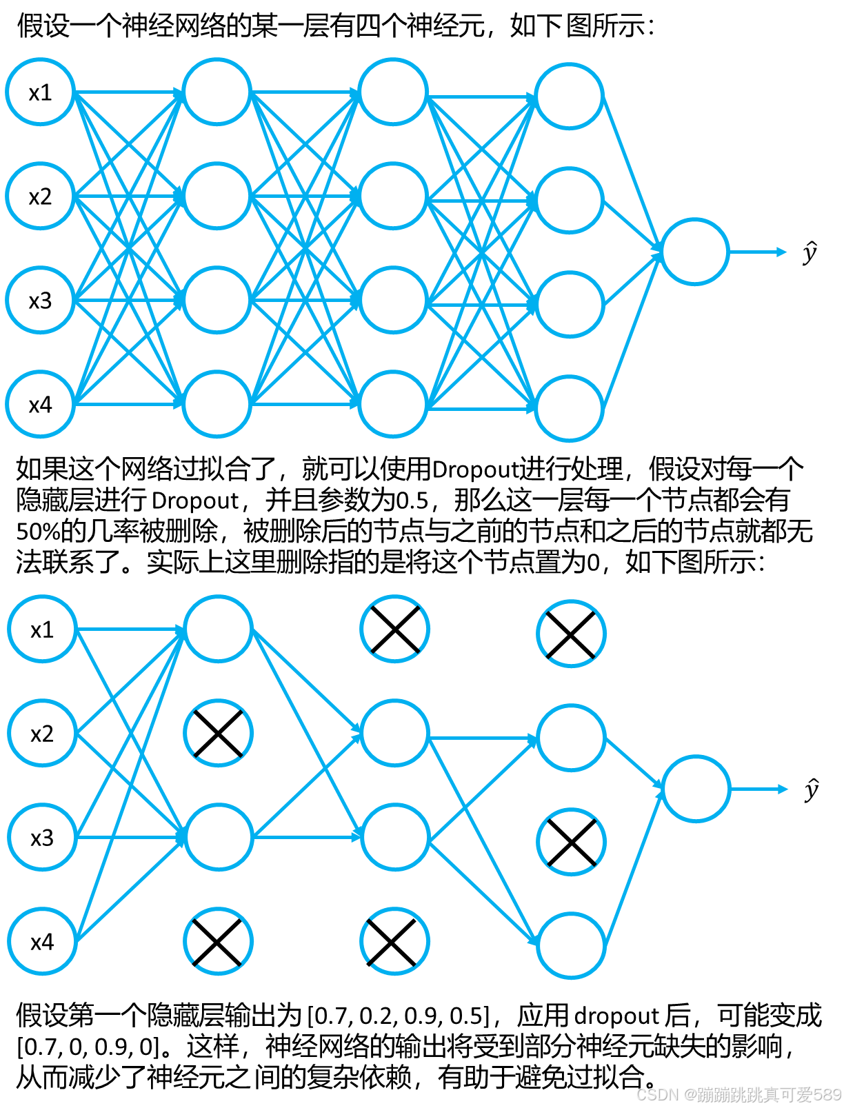
二、Dropout

        Dropout是一种在神经网络训练过程中使用的正则化技术，旨在减少过拟合现象。其 思想是在每次训练迭代中，随机地将一部分神经元的输出置为0，即将其“丢弃”，从 而降低神经网络对特定神经元的依赖性，减少神经网络的复杂度，增强神经网络的泛 化能力。

import torch  # 创建一个Dropout层，丢弃概率为0.2  
m = torch.nn.Dropout(p=0.2)  # 生成一个形状为(10, 1)的随机输入张量  
input = torch.randn(10, 1)  
print("输入张量:")  
print(input)  # 将Dropout层应用于输入张量  
output = m(input)  
print("应用Dropout后的输出:")  
print(output)  def dropout_layer(X, dropout):  # 确保dropout概率在0和1之间  assert 0 <= dropout <= 1  # 如果dropout为1，返回与X形状相同的全零张量  if dropout == 1:  return torch.zeros_like(X)  # 如果dropout为0，返回原始张量X  if dropout == 0:  return X  # 创建一个掩码，其中值大于指定的dropout概率  mask = (X > dropout).float()  print("掩码张量:")  print(mask)  # 通过掩码调整输出，并按dropout概率进行缩放  return mask * X / (1.0 - dropout)  # 将自定义dropout层应用于输入张量  
out = dropout_layer(input, 0.2)  
print("自定义dropout层的输出:")  
print(out)  

 Dropout为什么能够解决过拟合：

        （1）减少过拟合： 在标准的神经网络中，网络可能会过度依赖于一些特定的神经 元，导致对训练数据的过拟合。Dropout通过随机丢弃神经元，迫使网络学习对于任 何单个神经元的变化都要更加鲁棒的特征表示，从而减少了对训练数据的过度拟合。

        （2）取平均的作用： 在训练过程中，通过丢弃随机的神经元，每次前向传播都相当 于在训练不同的子网络。在测试阶段，不再进行Dropout，但是通过保留所有的权 重，网络结构变得更加完整。因此，可以看作是在多个不同的子网络中进行了训练， 最终的预测结果相当于对这些子网络的输出取平均。这种“综合取平均”的策略有助于 减轻过拟合，因为一些互为反向的拟合会相互抵消。

三、设计思路

输入数据

class1_points = np.array([[-0.7, 0.7], [3.9, 1.5], [1.7, 2.2], [1.9, -2.4], [0.9, 1.4], [4.2, 0.9], [1.7, 0.7], [0.2, -0.2], [3.1, -0.4],[-0.2, -0.9], [1.7, 0.2], [-0.6, -3.9], [-1.8, -4.0], [0.7, 3.8], [-0.7, -3.3], [0.8, 1.8], [-0.5, 1.5],[-0.6, -3.6], [-3.1, -3.0], [2.1, -2.5], [-2.5, -3.4], [-2.6, -0.8], [-0.2, 0.9], [-3.0, 3.3], [-0.7, 0.2],[0.3, 3.0], [0.6, 1.9], [-4.0, 2.4], [1.9, -2.2], [1.0, 0.3], [-0.9, -0.7], [-3.7, 0.6], [-2.7, -1.5], [0.9, -0.3],[0.8, -0.2], [-0.4, -4.4], [-0.3, 0.8], [4.1, 1.0], [-2.5, -3.5], [-0.8, 0.3], [0.6, 0.6], [2.6, -1.0], [1.8, 0.4],[1.5, -1.0], [3.2, 1.1], [3.3, -2.5], [-3.8, 2.5], [3.1, -0.9], [3.4, -1.1], [0.3, 0.8], [-0.1, 2.9], [-2.8, 1.9],[2.8, -3.3], [-1.0, 3.1], [-0.8, -0.6], [-2.5, -1.5], [0.3, 0.2], [-1.0, -2.9], [0.7, 0.2], [-0.5, 0.9],[-0.8, 0.7], [4.1, 0.5], [2.8, 2.3], [-3.9, 0.1], [2.2, -1.4], [-0.7, -3.5], [1.0, 1.2], [-0.7, -4.0], [1.3, 0.6],[-0.1, 3.3], [0.0, -0.3], [1.8, -3.0], [0.6, 0.0], [3.6, -2.8], [-3.9, -0.9], [-4.3, -0.9], [0.1, -0.8],[-1.6, -2.7], [-1.8, -3.3], [1.7, -3.5], [3.6, -3.1], [-2.4, 2.5], [-1.0, 1.8], [3.9, 2.5], [-3.9, -1.3],[3.4, 1.6], [-0.1, -0.6], [-3.7, -1.3], [-0.3, 3.4], [-3.7, -1.7], [4.0, 1.1], [3.4, 0.2], [0.1, -1.6],[-1.2, -0.5], [2.4, 1.7], [-4.4, -0.5], [-0.2, -3.6], [-0.8, 0.4], [-1.5, -2.2], [3.9, 2.5], [4.4, 1.4],[-3.5, -1.1], [-0.7, 1.5], [-3.0, -2.6], [0.2, -3.5], [0.0, 1.2], [-4.3, 0.1], [-1.8, 2.8], [1.1, -2.5],[0.2, 4.3], [-3.9, 2.2], [1.0, 1.6], [4.5, 0.2], [3.9, -1.6], [-0.4, -0.5], [0.3, -0.4], [-3.2, 1.7], [2.0, 4.1],[2.5, 2.2], [-1.1, -0.3], [-3.7, -1.9], [1.5, -1.1], [-2.1, -1.9], [-0.1, 4.5], [3.8, -0.3], [-0.9, -3.8],[-2.9, -1.6], [1.0, -1.2], [0.7, 0.0], [-0.8, 3.3], [-2.8, 3.1], [0.4, -3.2], [4.6, 1.0], [2.5, 3.1], [4.2, 0.8],[3.6, 1.8], [1.4, -3.0], [-0.4, -1.4], [-4.1, 1.1], [1.1, -0.2], [-2.9, -0.0], [-3.5, 1.3], [-1.4, 0.0],[-3.7, 2.2], [-2.9, 2.8], [1.7, 0.4], [-0.8, -0.6], [2.9, 1.1], [-2.3, 3.1], [-2.9, -2.0], [-2.7, -0.4],[2.6, -2.4], [-1.7, -2.8], [1.2, 3.1], [3.8, 1.3], [0.1, 1.9], [-0.5, -1.0], [0.0, -0.5], [3.9, -0.7],[-3.7, -2.5], [-3.1, 2.7], [-0.9, -1.0], [-0.7, -0.8], [-0.4, -0.1], [1.5, 1.0], [-2.6, 1.9], [-0.8, 1.7],[0.8, 1.8], [2.0, 3.6], [3.2, 1.4], [2.3, 1.4], [4.9, 0.5], [2.2, 1.8], [-1.4, -2.7], [3.1, 1.1], [-1.0, 3.8],[-0.4, -1.1], [3.3, 1.1], [2.2, -3.9], [1.0, 1.2], [2.6, 3.2], [-0.6, -3.0], [-1.9, -2.8], [1.2, -1.2],[-0.4, -2.7], [1.1, -4.3], [0.3, -0.8], [-1.0, -0.4], [-1.1, -0.2], [0.1, 1.2], [0.9, 0.6], [-2.7, 1.6],[1.0, -0.7], [0.3, -4.2], [-2.1, 3.2], [3.4, -1.2], [2.5, -4.0], [1.0, -0.8], [1.0, -0.9], [0.1, -0.6]])
class2_points = np.array([[-3.0, -3.8], [4.4, 2.5], [2.6, 4.1], [3.7, -2.7], [-3.7, -2.9], [5.3, 0.3], [3.9, 2.9], [-2.7, -4.5], [5.4, 0.2],[3.0, 4.8], [-4.2, -1.3], [-2.1, -5.4], [-3.2, -4.6], [0.7, 4.5], [-1.4, -5.7], [0.5, 5.9], [-2.1, 4.0],[-0.1, -5.1], [-3.4, -4.7], [3.3, -4.7], [-2.7, -4.1], [-4.5, -2.0], [4.3, 2.9], [-3.6, 4.0], [-0.5, 5.5],[0.2, 5.2], [5.3, -0.9], [-4.5, 3.6], [3.4, -2.8], [-3.4, -3.7], [1.6, -5.5], [-5.9, -0.1], [-4.8, -2.5],[-5.5, 0.3], [1.6, 4.4], [-0.9, -5.3], [-1.0, 5.4], [4.9, 0.8], [-3.1, -4.0], [2.3, 4.7], [4.0, -1.6], [4.9, -1.5],[4.2, -2.5], [-3.5, 3.7], [4.7, 0.5], [5.3, -2.6], [-5.0, 2.4], [5.5, -1.2], [5.6, -1.3], [3.3, -4.3], [-1.3, 4.4],[-4.1, 3.6], [3.3, -4.5], [-2.3, 5.2], [2.6, 4.6], [-4.4, -1.6], [4.7, -2.0], [-1.7, -4.9], [-5.1, -2.4],[4.5, 3.2], [-3.9, -3.4], [6.0, -0.4], [3.5, 4.3], [-4.9, -0.6], [3.3, -3.2], [-0.3, -4.8], [-1.6, -4.7],[-1.4, -4.6], [-3.1, 3.8], [-1.4, 4.9], [1.8, -4.5], [2.2, -5.5], [3.1, -3.4], [4.7, -2.8], [-5.3, -0.4],[-6.0, -0.1], [1.4, -4.5], [-3.1, -4.3], [-1.8, -5.7], [1.7, -5.6], [4.5, -3.7], [-2.6, 4.3], [-3.4, 3.4],[4.7, 3.1], [-5.2, -2.8], [5.4, 1.2], [-5.4, 1.2], [-4.9, -1.3], [-1.3, 5.6], [-4.1, -2.6], [5.0, 1.0], [5.2, 1.2],[2.4, -4.9], [-3.2, 3.8], [3.3, 3.4], [-5.5, -0.8], [0.6, -5.0], [1.2, 5.4], [-3.4, -3.3], [4.6, 2.8], [5.2, 1.7],[-4.4, -0.9], [-5.0, -1.3], [-3.1, -3.6], [-0.7, -4.5], [5.9, -0.9], [-5.1, -0.5], [-2.6, 5.2], [1.4, -4.8],[-0.7, 5.6], [-5.3, 2.1], [4.9, 2.6], [5.3, 0.9], [5.1, -1.2], [2.7, -4.4], [-2.0, -5.6], [-4.9, 3.2], [2.8, 5.3],[2.6, 3.9], [-0.0, 5.7], [-5.7, -1.8], [-1.1, -4.7], [-2.4, -3.8], [-1.1, 5.6], [5.3, -1.5], [-0.4, -5.8],[-4.5, -1.6], [-4.4, -3.7], [-4.3, 2.4], [0.1, 4.8], [-3.0, 3.8], [0.3, -5.8], [5.6, 0.5], [4.1, 3.6], [5.0, 1.5],[5.7, 1.5], [3.2, -4.1], [-1.7, -5.6], [-5.3, 0.9], [4.3, 3.0], [-5.4, 0.3], [-5.0, 0.8], [2.7, 5.1], [-5.0, 2.2],[-4.0, 3.0], [-4.4, -3.9], [-3.5, -3.9], [5.3, 1.5], [-4.2, 4.2], [-3.9, -4.0], [-4.7, -0.1], [3.7, -4.7],[-3.0, -4.7], [2.7, 4.4], [4.3, 2.0], [-3.6, -4.5], [5.5, 0.9], [-4.7, -2.8], [5.5, -2.2], [-5.1, -2.6],[-3.6, 3.1], [-3.2, -4.0], [-4.8, 1.3], [-5.5, -1.6], [4.1, -1.6], [-4.2, 3.6], [5.6, -1.4], [4.9, -3.3],[1.7, 4.9], [5.3, 2.5], [3.8, 2.8], [5.8, 0.7], [3.9, 2.6], [-2.1, -4.8], [5.2, 2.5], [-2.0, 4.3], [2.8, -4.1],[5.6, 0.8], [2.2, -5.2], [-1.1, 5.5], [4.2, 3.8], [-1.8, -5.2], [-3.4, -3.6], [3.7, -3.6], [-0.5, -4.8],[1.9, -5.6], [-1.1, 5.4], [2.3, 4.7], [0.0, -5.4], [2.1, -5.6], [4.8, -0.3], [-4.7, 2.9], [-3.8, 3.9], [0.9, -5.5],[-2.3, 3.6], [5.3, -2.5], [3.7, -4.6], [-5.0, 2.4], [0.0, -5.7], [0.2, -5.9]])# 合并两类点
points = np.concatenate((class1_points, class2_points))
# 标签 0表示类别1，1表示类别2
labels1 = np.zeros(len(class1_points))
labels2 = np.ones(len(class2_points))labels = np.concatenate((labels1, labels2))

构建模型

class ModelClass(nn.Module):def __init__(self):super().__init__()# 定义网络层结构：self.layer1 = nn.Linear(2, 16)  # 输入层（2维特征）→ 16维隐藏层self.layer2 = nn.Linear(16, 48)  # 16维 → 48维隐藏层self.layer3 = nn.Linear(48, 32)  # 48维 → 32维隐藏层self.layer4 = nn.Linear(32, 2)  # 32维 → 输出层（2类概率）# 定义Dropout层（随机丢弃神经元防止过拟合）self.dropout1 = nn.Dropout(p=0.1)  # 丢弃概率10%self.dropout2 = nn.Dropout(p=0.1)self.dropout3 = nn.Dropout(p=0.1)def forward(self, x):x = torch.relu(self.layer1(x))  # 第一层后接ReLU激活函数x = self.dropout1(x)  # 应用Dropoutx = torch.relu(self.layer2(x))  # 第二层 + ReLUx = self.dropout2(x)x = torch.relu(self.layer3(x))  # 第三层 + ReLUx = self.dropout3(x)x=self.layer4(x) # 输出层Softmax获取概率return x# 初始化模型实例
model = ModelClass()

构建损失函数和优化器

criterion = nn.CrossEntropyLoss()  # 交叉熵损失函数（多分类任务常用）
optimizer = optim.Adam(model.parameters(), lr=0.01)  # Adam优化器，学习率0.01

 训练模型

num_iterations = 2000  # 总迭代次数
batch_size = 32  # 批量大小for n in range(num_iterations + 1):model.train()  # 设置模型为训练模式（启用Dropout）# 分批训练for batch_start in range(0, len(points), batch_size):# 获取当前批次的数据和标签batch_inputs = torch.tensor(points[batch_start:batch_start + batch_size], dtype=torch.float32)batch_labels = torch.tensor(labels[batch_start:batch_start + batch_size], dtype=torch.long)# 前向传播outputs = model(batch_inputs)loss = criterion(outputs, batch_labels)  # 计算损失# 反向传播与优化optimizer.zero_grad()  # 清空梯度缓存loss.backward()  # 反向传播计算梯度optimizer.step()  # 更新权重参数# 每隔100次迭代可视化结果if n % 100 == 0 or n == 1:print(n,loss.item())

可视化

num_iterations = 2000  # 总迭代次数
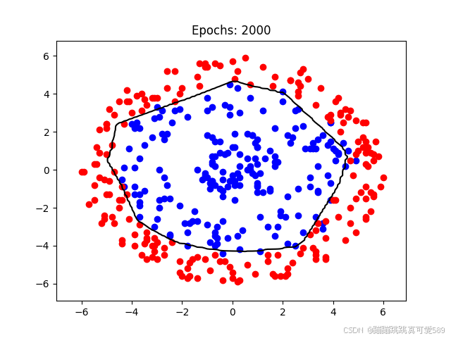
batch_size = 32  # 批量大小for n in range(num_iterations + 1):model.train()  # 设置模型为训练模式（启用Dropout）# 分批训练for batch_start in range(0, len(points), batch_size):# 获取当前批次的数据和标签batch_inputs = torch.tensor(points[batch_start:batch_start + batch_size], dtype=torch.float32)batch_labels = torch.tensor(labels[batch_start:batch_start + batch_size], dtype=torch.long)# 前向传播outputs = model(batch_inputs)loss = criterion(outputs, batch_labels)  # 计算损失# 反向传播与优化optimizer.zero_grad()  # 清空梯度缓存loss.backward()  # 反向传播计算梯度optimizer.step()  # 更新权重参数# 每隔100次迭代可视化结果if n % 100 == 0 or n == 1:print(n,loss.item())model.eval()  # 设置模型为评估模式（关闭Dropout）with torch.no_grad():  # 关闭梯度计算# 预测所有网格点的类别概率grid_points_tensor = torch.tensor(grid_points, dtype=torch.float32)Z = model(grid_points_tensor).numpy()Z = Z[:, 1]  # 获取类别2的概率值# 调整形状以匹配网格矩阵Z = Z.reshape(xx.shape)# 绘制分类结果plt.cla()  # 清空当前图像plt.scatter(class1_points[:, 0], class1_points[:, 1], c='blue', label='Class 1')plt.scatter(class2_points[:, 0], class2_points[:, 1], c='red', label='Class 2')plt.contour(xx, yy, Z, levels=[0.5], colors='black')  # 绘制0.5概率等高线作为决策边界plt.title(f"Epochs: {n}")plt.show()  # 显示最终图像

完整代码

import numpy as np
import torch
import torch.nn as nn
import torch.optim as optim
import matplotlib.pyplot as plt# --------------------------------------------- 数据准备部分 ---------------------------------------------
# 类别1的二维坐标点（蓝色点）
class1_points = np.array([[-0.7, 0.7], [3.9, 1.5], [1.7, 2.2], [1.9, -2.4], [0.9, 1.4], [4.2, 0.9], [1.7, 0.7], [0.2, -0.2], [3.1, -0.4],[-0.2, -0.9], [1.7, 0.2], [-0.6, -3.9], [-1.8, -4.0], [0.7, 3.8], [-0.7, -3.3], [0.8, 1.8], [-0.5, 1.5],[-0.6, -3.6], [-3.1, -3.0], [2.1, -2.5], [-2.5, -3.4], [-2.6, -0.8], [-0.2, 0.9], [-3.0, 3.3], [-0.7, 0.2],[0.3, 3.0], [0.6, 1.9], [-4.0, 2.4], [1.9, -2.2], [1.0, 0.3], [-0.9, -0.7], [-3.7, 0.6], [-2.7, -1.5], [0.9, -0.3],[0.8, -0.2], [-0.4, -4.4], [-0.3, 0.8], [4.1, 1.0], [-2.5, -3.5], [-0.8, 0.3], [0.6, 0.6], [2.6, -1.0], [1.8, 0.4],[1.5, -1.0], [3.2, 1.1], [3.3, -2.5], [-3.8, 2.5], [3.1, -0.9], [3.4, -1.1], [0.3, 0.8], [-0.1, 2.9], [-2.8, 1.9],[2.8, -3.3], [-1.0, 3.1], [-0.8, -0.6], [-2.5, -1.5], [0.3, 0.2], [-1.0, -2.9], [0.7, 0.2], [-0.5, 0.9],[-0.8, 0.7], [4.1, 0.5], [2.8, 2.3], [-3.9, 0.1], [2.2, -1.4], [-0.7, -3.5], [1.0, 1.2], [-0.7, -4.0], [1.3, 0.6],[-0.1, 3.3], [0.0, -0.3], [1.8, -3.0], [0.6, 0.0], [3.6, -2.8], [-3.9, -0.9], [-4.3, -0.9], [0.1, -0.8],[-1.6, -2.7], [-1.8, -3.3], [1.7, -3.5], [3.6, -3.1], [-2.4, 2.5], [-1.0, 1.8], [3.9, 2.5], [-3.9, -1.3],[3.4, 1.6], [-0.1, -0.6], [-3.7, -1.3], [-0.3, 3.4], [-3.7, -1.7], [4.0, 1.1], [3.4, 0.2], [0.1, -1.6],[-1.2, -0.5], [2.4, 1.7], [-4.4, -0.5], [-0.2, -3.6], [-0.8, 0.4], [-1.5, -2.2], [3.9, 2.5], [4.4, 1.4],[-3.5, -1.1], [-0.7, 1.5], [-3.0, -2.6], [0.2, -3.5], [0.0, 1.2], [-4.3, 0.1], [-1.8, 2.8], [1.1, -2.5],[0.2, 4.3], [-3.9, 2.2], [1.0, 1.6], [4.5, 0.2], [3.9, -1.6], [-0.4, -0.5], [0.3, -0.4], [-3.2, 1.7], [2.0, 4.1],[2.5, 2.2], [-1.1, -0.3], [-3.7, -1.9], [1.5, -1.1], [-2.1, -1.9], [-0.1, 4.5], [3.8, -0.3], [-0.9, -3.8],[-2.9, -1.6], [1.0, -1.2], [0.7, 0.0], [-0.8, 3.3], [-2.8, 3.1], [0.4, -3.2], [4.6, 1.0], [2.5, 3.1], [4.2, 0.8],[3.6, 1.8], [1.4, -3.0], [-0.4, -1.4], [-4.1, 1.1], [1.1, -0.2], [-2.9, -0.0], [-3.5, 1.3], [-1.4, 0.0],[-3.7, 2.2], [-2.9, 2.8], [1.7, 0.4], [-0.8, -0.6], [2.9, 1.1], [-2.3, 3.1], [-2.9, -2.0], [-2.7, -0.4],[2.6, -2.4], [-1.7, -2.8], [1.2, 3.1], [3.8, 1.3], [0.1, 1.9], [-0.5, -1.0], [0.0, -0.5], [3.9, -0.7],[-3.7, -2.5], [-3.1, 2.7], [-0.9, -1.0], [-0.7, -0.8], [-0.4, -0.1], [1.5, 1.0], [-2.6, 1.9], [-0.8, 1.7],[0.8, 1.8], [2.0, 3.6], [3.2, 1.4], [2.3, 1.4], [4.9, 0.5], [2.2, 1.8], [-1.4, -2.7], [3.1, 1.1], [-1.0, 3.8],[-0.4, -1.1], [3.3, 1.1], [2.2, -3.9], [1.0, 1.2], [2.6, 3.2], [-0.6, -3.0], [-1.9, -2.8], [1.2, -1.2],[-0.4, -2.7], [1.1, -4.3], [0.3, -0.8], [-1.0, -0.4], [-1.1, -0.2], [0.1, 1.2], [0.9, 0.6], [-2.7, 1.6],[1.0, -0.7], [0.3, -4.2], [-2.1, 3.2], [3.4, -1.2], [2.5, -4.0], [1.0, -0.8], [1.0, -0.9], [0.1, -0.6]])
class2_points = np.array([[-3.0, -3.8], [4.4, 2.5], [2.6, 4.1], [3.7, -2.7], [-3.7, -2.9], [5.3, 0.3], [3.9, 2.9], [-2.7, -4.5], [5.4, 0.2],[3.0, 4.8], [-4.2, -1.3], [-2.1, -5.4], [-3.2, -4.6], [0.7, 4.5], [-1.4, -5.7], [0.5, 5.9], [-2.1, 4.0],[-0.1, -5.1], [-3.4, -4.7], [3.3, -4.7], [-2.7, -4.1], [-4.5, -2.0], [4.3, 2.9], [-3.6, 4.0], [-0.5, 5.5],[0.2, 5.2], [5.3, -0.9], [-4.5, 3.6], [3.4, -2.8], [-3.4, -3.7], [1.6, -5.5], [-5.9, -0.1], [-4.8, -2.5],[-5.5, 0.3], [1.6, 4.4], [-0.9, -5.3], [-1.0, 5.4], [4.9, 0.8], [-3.1, -4.0], [2.3, 4.7], [4.0, -1.6], [4.9, -1.5],[4.2, -2.5], [-3.5, 3.7], [4.7, 0.5], [5.3, -2.6], [-5.0, 2.4], [5.5, -1.2], [5.6, -1.3], [3.3, -4.3], [-1.3, 4.4],[-4.1, 3.6], [3.3, -4.5], [-2.3, 5.2], [2.6, 4.6], [-4.4, -1.6], [4.7, -2.0], [-1.7, -4.9], [-5.1, -2.4],[4.5, 3.2], [-3.9, -3.4], [6.0, -0.4], [3.5, 4.3], [-4.9, -0.6], [3.3, -3.2], [-0.3, -4.8], [-1.6, -4.7],[-1.4, -4.6], [-3.1, 3.8], [-1.4, 4.9], [1.8, -4.5], [2.2, -5.5], [3.1, -3.4], [4.7, -2.8], [-5.3, -0.4],[-6.0, -0.1], [1.4, -4.5], [-3.1, -4.3], [-1.8, -5.7], [1.7, -5.6], [4.5, -3.7], [-2.6, 4.3], [-3.4, 3.4],[4.7, 3.1], [-5.2, -2.8], [5.4, 1.2], [-5.4, 1.2], [-4.9, -1.3], [-1.3, 5.6], [-4.1, -2.6], [5.0, 1.0], [5.2, 1.2],[2.4, -4.9], [-3.2, 3.8], [3.3, 3.4], [-5.5, -0.8], [0.6, -5.0], [1.2, 5.4], [-3.4, -3.3], [4.6, 2.8], [5.2, 1.7],[-4.4, -0.9], [-5.0, -1.3], [-3.1, -3.6], [-0.7, -4.5], [5.9, -0.9], [-5.1, -0.5], [-2.6, 5.2], [1.4, -4.8],[-0.7, 5.6], [-5.3, 2.1], [4.9, 2.6], [5.3, 0.9], [5.1, -1.2], [2.7, -4.4], [-2.0, -5.6], [-4.9, 3.2], [2.8, 5.3],[2.6, 3.9], [-0.0, 5.7], [-5.7, -1.8], [-1.1, -4.7], [-2.4, -3.8], [-1.1, 5.6], [5.3, -1.5], [-0.4, -5.8],[-4.5, -1.6], [-4.4, -3.7], [-4.3, 2.4], [0.1, 4.8], [-3.0, 3.8], [0.3, -5.8], [5.6, 0.5], [4.1, 3.6], [5.0, 1.5],[5.7, 1.5], [3.2, -4.1], [-1.7, -5.6], [-5.3, 0.9], [4.3, 3.0], [-5.4, 0.3], [-5.0, 0.8], [2.7, 5.1], [-5.0, 2.2],[-4.0, 3.0], [-4.4, -3.9], [-3.5, -3.9], [5.3, 1.5], [-4.2, 4.2], [-3.9, -4.0], [-4.7, -0.1], [3.7, -4.7],[-3.0, -4.7], [2.7, 4.4], [4.3, 2.0], [-3.6, -4.5], [5.5, 0.9], [-4.7, -2.8], [5.5, -2.2], [-5.1, -2.6],[-3.6, 3.1], [-3.2, -4.0], [-4.8, 1.3], [-5.5, -1.6], [4.1, -1.6], [-4.2, 3.6], [5.6, -1.4], [4.9, -3.3],[1.7, 4.9], [5.3, 2.5], [3.8, 2.8], [5.8, 0.7], [3.9, 2.6], [-2.1, -4.8], [5.2, 2.5], [-2.0, 4.3], [2.8, -4.1],[5.6, 0.8], [2.2, -5.2], [-1.1, 5.5], [4.2, 3.8], [-1.8, -5.2], [-3.4, -3.6], [3.7, -3.6], [-0.5, -4.8],[1.9, -5.6], [-1.1, 5.4], [2.3, 4.7], [0.0, -5.4], [2.1, -5.6], [4.8, -0.3], [-4.7, 2.9], [-3.8, 3.9], [0.9, -5.5],[-2.3, 3.6], [5.3, -2.5], [3.7, -4.6], [-5.0, 2.4], [0.0, -5.7], [0.2, -5.9]])# 合并两类点
points = np.concatenate((class1_points, class2_points))
# 标签 0表示类别1，1表示类别2
labels1 = np.zeros(len(class1_points))
labels2 = np.ones(len(class2_points))labels = np.concatenate((labels1, labels2))# --------------------------------------------- 模型定义部分 ---------------------------------------------
class ModelClass(nn.Module):def __init__(self):super().__init__()# 定义网络层结构：self.layer1 = nn.Linear(2, 16)  # 输入层（2维特征）→ 16维隐藏层self.layer2 = nn.Linear(16, 48)  # 16维 → 48维隐藏层self.layer3 = nn.Linear(48, 32)  # 48维 → 32维隐藏层self.layer4 = nn.Linear(32, 2)  # 32维 → 输出层（2类概率）# 定义Dropout层（随机丢弃神经元防止过拟合）self.dropout1 = nn.Dropout(p=0.1)  # 丢弃概率10%self.dropout2 = nn.Dropout(p=0.1)self.dropout3 = nn.Dropout(p=0.1)def forward(self, x):x = torch.relu(self.layer1(x))  # 第一层后接ReLU激活函数x = self.dropout1(x)  # 应用Dropoutx = torch.relu(self.layer2(x))  # 第二层 + ReLUx = self.dropout2(x)x = torch.relu(self.layer3(x))  # 第三层 + ReLUx = self.dropout3(x)x=self.layer4(x) # 输出层Softmax获取概率return x# 初始化模型实例
model = ModelClass()
# --------------------------------------------- 训练配置部分 ---------------------------------------------
criterion = nn.CrossEntropyLoss()  # 交叉熵损失函数（多分类任务常用）
optimizer = optim.Adam(model.parameters(), lr=0.01)  # Adam优化器，学习率0.01# 生成网格点用于绘制决策边界
x_min, x_max = points[:, 0].min() - 1, points[:, 0].max() + 1
y_min, y_max = points[:, 1].min() - 1, points[:, 1].max() + 1
step_size = 0.1
xx, yy = np.meshgrid(np.arange(x_min, x_max, step_size),np.arange(y_min, y_max, step_size))
grid_points = np.c_[xx.ravel(), yy.ravel()]  # 生成网格坐标矩阵# --------------------------------------------- 训练循环部分 ---------------------------------------------
num_iterations = 2000  # 总迭代次数
batch_size = 32  # 批量大小for n in range(num_iterations + 1):model.train()  # 设置模型为训练模式（启用Dropout）# 分批训练for batch_start in range(0, len(points), batch_size):# 获取当前批次的数据和标签batch_inputs = torch.tensor(points[batch_start:batch_start + batch_size], dtype=torch.float32)batch_labels = torch.tensor(labels[batch_start:batch_start + batch_size], dtype=torch.long)# 前向传播outputs = model(batch_inputs)loss = criterion(outputs, batch_labels)  # 计算损失# 反向传播与优化optimizer.zero_grad()  # 清空梯度缓存loss.backward()  # 反向传播计算梯度optimizer.step()  # 更新权重参数# 每隔100次迭代可视化结果if n % 100 == 0 or n == 1:print(n,loss.item())model.eval()  # 设置模型为评估模式（关闭Dropout）with torch.no_grad():  # 关闭梯度计算# 预测所有网格点的类别概率grid_points_tensor = torch.tensor(grid_points, dtype=torch.float32)Z = model(grid_points_tensor).numpy()Z = Z[:, 1]  # 获取类别2的概率值# 调整形状以匹配网格矩阵Z = Z.reshape(xx.shape)# 绘制分类结果plt.cla()  # 清空当前图像plt.scatter(class1_points[:, 0], class1_points[:, 1], c='blue', label='Class 1')plt.scatter(class2_points[:, 0], class2_points[:, 1], c='red', label='Class 2')plt.contour(xx, yy, Z, levels=[0.5], colors='black')  # 绘制0.5概率等高线作为决策边界plt.title(f"Epochs: {n}")plt.show()  # 显示最终图像