当前位置：首页 > news >正文

记录一下线性回归的学习

news 来源：原创 2025/4/24 12:15:09

一、线性回归的定义

线性回归（Linear regression）用来建模和分析变量之间线性关系，适用于预测连续性目标变量。它通过拟合成一条线来描述自变量和因变量之间的线性关系。自变量可以有多个，只有一个自变量的时候，成为单变量回归，自变量多于一个时，成为多元回归。

通用的公式为：

$y = \beta_{0} + \beta _{1}x_{1} + \beta _{2}x_{2} + \beta _{3}x_{3} + \cdots + \beta _{n}x_{n}$

其中 y 表示因变量，x 表示自变量，下标 n 是表示有几个因变量。 $\beta_{0}\cdots \beta_{n}$ 表示回归系数， $\beta _{0}$ 表示拟合出来的线的截距。

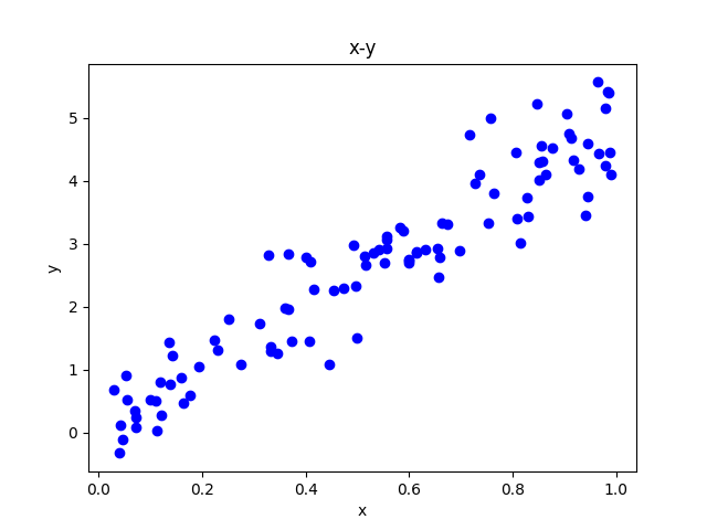
使用线性回归来预测目标变量的前提是，因变量和自变量呈现线性的关系，如下图：

二、代码实现

1、使用到的库：

sklearn：是一个用于机器学习的python开源库，具有丰富的机器学习算法和工具，防范用于数据挖掘、数据分析、测试建模等领域。

（1）算法方面：涵盖了分类、回归、聚类、降维等多种机器学习。

（2）提供一些列数据预处理工具。

（3）多种评估指标和模型选择方法。

（4）使用joblib或者pickle模块可以将训练好的模型参数保存下来。

matplotlib：一个功能强大的python绘图库，主要用于数据的可视化。

2、代码实现：

（1）单变量回归，只有一个自变量

import pickle
from matplotlib import pyplot as plt
from skimage.metrics import mean_squared_error
from sklearn.model_selection import train_test_split
from sklearn.linear_model import LinearRegression
import numpy as np# 随机生成数据
def load_data():x_data = np.random.rand(100, 1)y = x_data * 5 + 0.5 * np.random.randn(100, 1)x_train, x_val, y_train, y_val = train_test_split(x_data, y, test_size=0.2)return x_train, x_val, y_train, y_val# 绘制预测结果与真是标签的散点图
def draw_result(y_test, y_pred):plt.scatter(y_test, y_pred, color='blue')plt.plot([min(y_pred), max(y_pred)], [min(y_pred), max(y_pred)], linestyle='--', color='red', linewidth=2,label='Regression Line')plt.title('Actual vs Predicted Profit')plt.xlabel('Actual Profit')plt.ylabel('Predicted Profit')plt.show()def train(x_train, x_test, y_train, y_test):model = LinearRegression()# 训练模型model.fit(x_train, y_train)# 对验证集测试y_pred = model.predict(x_test)mse = mean_squared_error(y_test, y_pred)print(f'误差为:{mse}')# 绘制结果的散点图draw_result(y_test, y_pred)# 保存模型with open('model.pkl', 'wb') as f_model:pickle.dump(model, f_model)# 使用训练出来的模型推理新数据
def predict(x_test, y_test):with open('model.pkl', 'rb') as file:model_best = pickle.load(file)pred = model_best.predict(x_test)draw_result(y_test, pred)return predif __name__ == '__main__':# 生成数据x_train, x_val, y_train, y_val = load_data()# 训练train(x_train, x_val, y_train, y_val)# 生成测试数据x_test_data = np.random.rand(10,1)y_test_data = x_test_data * 5 + 0.5 * np.random.randn(10, 1)# 推理predict_result = predict(x_test_data, y_test_data)

（2）多元回归，只需要将x的数据修改成多元的就可以了，其他的都是一样的。

import pickle
from matplotlib import pyplot as plt
from skimage.metrics import mean_squared_error
from sklearn.model_selection import train_test_split
from sklearn.linear_model import LinearRegression
import numpy as np# 随机生成数据
def load_data():x_data = np.random.rand(100, 2)y = 5 * x_data[:, 0:1] + 3 * x_data[:, 1:2] + 0.5 * np.random.randn(100, 1)x_train, x_val, y_train, y_val = train_test_split(x_data, y, test_size=0.2)return x_train, x_val, y_train, y_val# 绘制预测结果与真是标签的散点图
def draw_result(y_test, y_pred):plt.scatter(y_test, y_pred, color='blue')plt.plot([min(y_pred), max(y_pred)], [min(y_pred), max(y_pred)], linestyle='--', color='red', linewidth=2,label='Regression Line')plt.title('Actual vs Predicted Profit')plt.xlabel('Actual Profit')plt.ylabel('Predicted Profit')plt.show()def train(x_train, x_test, y_train, y_test):model = LinearRegression()# 训练模型model.fit(x_train, y_train)# 对验证集测试y_pred = model.predict(x_test)mse = mean_squared_error(y_test, y_pred)print(f'误差为:{mse}')print(y_pred.shape)print(y_test.shape)# 绘制结果的散点图draw_result(y_test, y_pred)# 保存模型with open('model.pkl', 'wb') as f_model:pickle.dump(model, f_model)# 使用训练出来的模型推理新数据
def predict(x_test, y_test):with open('model.pkl', 'rb') as file:model_best = pickle.load(file)pred = model_best.predict(x_test)draw_result(y_test, pred)return predif __name__ == '__main__':# 生成数据x_train, x_val, y_train, y_val = load_data()# 训练train(x_train, x_val, y_train, y_val)# 生成测试数据x_test_data = np.random.rand(10,2)y_test_data = x_test_data[:, 0:1] * 5 + x_test_data[:, 1:2] * 3 + 0.5 * np.random.randn(10, 1)# 推理predict_result = predict(x_test_data, y_test_data)