day9 python 热力图与子图的绘制
在数据分析过程中,热力图和子图是非常实用的可视化工具,能够帮助我们更直观地理解数据之间的关系和特征分布。本文将结合实际数据,详细介绍如何使用 Python 绘制热力图和子图。
一、数据读取与初步处理
首先,我们需要读取数据文件。这里假设数据存储在名为 data.csv 的文件中,使用 pandas 库的 read_csv 函数进行读取:
import pandas as pd
data = pd.read_csv('data.csv')
读取数据后,我们可以使用 info 方法查看数据的基本信息,包括数据的行数、列数、每列的数据类型以及缺失值的情况:
data.info()
输出结果如下:
<class 'pandas.core.frame.DataFrame'>
RangeIndex: 7500 entries, 0 to 7499
Data columns (total 18 columns):#   Column                        Non-Null Count  Dtype
---  ------                        --------------  -----  0   Id                            7500 non-null   int64  1   Home Ownership                7500 non-null   object 2   Annual Income                 5943 non-null   float643   Years in current job          7129 non-null   object 4   Tax Liens                     7500 non-null   float645   Number of Open Accounts       7500 non-null   float646   Years of Credit History       7500 non-null   float647   Maximum Open Credit           7500 non-null   float648   Number of Credit Problems     7500 non-null   float649   Months since last delinquent  3419 non-null   float6410  Bankruptcies                  7486 non-null   float6411  Purpose                       7500 non-null   object 12  Term                          7500 non-null   object 13  Current Loan Amount           7500 non-null   float6414  Current Credit Balance        7500 non-null   float6415  Monthly Debt                  7500 non-null   float6416  Credit Score                  5943 non-null   float6417  Credit Default                7500 non-null   int64
dtypes: float64(12), int64(2), object(4)
memory usage: 1.0+ MB
同时,使用 head 方法查看数据的前几行:
data.head(5)
输出结果:
| Id | Home Ownership | Annual Income | Years in current job | Tax Liens | Number of Open Accounts | Years of Credit History | Maximum Open Credit | Number of Credit Problems | Months since last delinquent | Bankruptcies | Purpose | Term | Current Loan Amount | Current Credit Balance | Monthly Debt | Credit Score | Credit Default | |
|---|---|---|---|---|---|---|---|---|---|---|---|---|---|---|---|---|---|---|
| 0 | 0 | Own Home | 482087.0 | NaN | 0.0 | 11.0 | 26.3 | 685960.0 | 1.0 | NaN | 1.0 | debt consolidation | Short Term | 99999999.0 | 47386.0 | 7914.0 | 749.0 | 0 |
| 1 | 1 | Own Home | 1025487.0 | 10+ years | 0.0 | 15.0 | 15.3 | 1181730.0 | 0.0 | NaN | 0.0 | debt consolidation | Long Term | 264968.0 | 394972.0 | 18373.0 | 737.0 | 1 |
| 2 | 2 | Home Mortgage | 751412.0 | 8 years | 0.0 | 11.0 | 35.0 | 1182434.0 | 0.0 | NaN | 0.0 | debt consolidation | Short Term | 99999999.0 | 308389.0 | 13651.0 | 742.0 | 0 |
| 3 | 3 | Own Home | 805068.0 | 6 years | 0.0 | 8.0 | 22.5 | 147400.0 | 1.0 | NaN | 1.0 | debt consolidation | Short Term | 121396.0 | 95855.0 | 11338.0 | 694.0 | 0 |
| 4 | 4 | Rent | 776264.0 | 8 years | 0.0 | 13.0 | 13.6 | 385836.0 | 1.0 | NaN | 0.0 | debt consolidation | Short Term | 125840.0 | 93309.0 | 7180.0 | 719.0 | 0 |
为了后续分析的方便,我们需要将 Years in current job 列和 Home Ownership 列的字符串类型数据转化为数字类型。
先查看这两列数据的具体取值分布:
data["Years in current job"].value_counts()
10+ years    2332
2 years       705
3 years       620
< 1 year      563
5 years       516
1 year        504
4 years       469
6 years       426
7 years       396
8 years       339
9 years       259
Name: Years in current job, dtype: int64
data["Home Ownership"].value_counts()
Home Mortgage    3637
Rent             3204
Own Home          647
Have Mortgage      12
Name: Home Ownership, dtype: int64
然后创建映射字典进行转换:
mappings = {"Years in current job": {"10+ years": 10,"2 years": 2,"3 years": 3,"< 1 year": 0,"5 years": 5,"1 year": 1,"4 years": 4,"6 years": 6,"7 years": 7,"8 years": 8,"9 years": 9},"Home Ownership": {"Home Mortgage": 0,"Rent": 1,"Own Home": 2,"Have Mortgage": 3}
}
data["Years in current job"] = data["Years in current job"].map(mappings["Years in current job"])
data["Home Ownership"] = data["Home Ownership"].map(mappings["Home Ownership"])
再次查看数据信息:
data.info()
输出结果:
<class 'pandas.core.frame.DataFrame'>
RangeIndex: 7500 entries, 0 to 7499
Data columns (total 18 columns):#   Column                        Non-Null Count  Dtype
---  ------                        --------------  -----  0   Id                            7500 non-null   int64  1   Home Ownership                7500 non-null   int64  2   Annual Income                 5943 non-null   float643   Years in current job          7129 non-null   float644   Tax Liens                     7500 non-null   float645   Number of Open Accounts       7500 non-null   float646   Years of Credit History       7500 non-null   float647   Maximum Open Credit           7500 non-null   float648   Number of Credit Problems     7500 non-null   float649   Months since last delinquent  3419 non-null   float6410  Bankruptcies                  7486 non-null   float6411  Purpose                       7500 non-null   object 12  Term                          7500 non-null   object 13  Current Loan Amount           7500 non-null   float6414  Current Credit Balance        7500 non-null   float6415  Monthly Debt                  7500 non-null   float6416  Credit Score                  5943 non-null   float6417  Credit Default                7500 non-null   int64
dtypes: float64(13), int64(3), object(2)
memory usage: 1.0+ MB
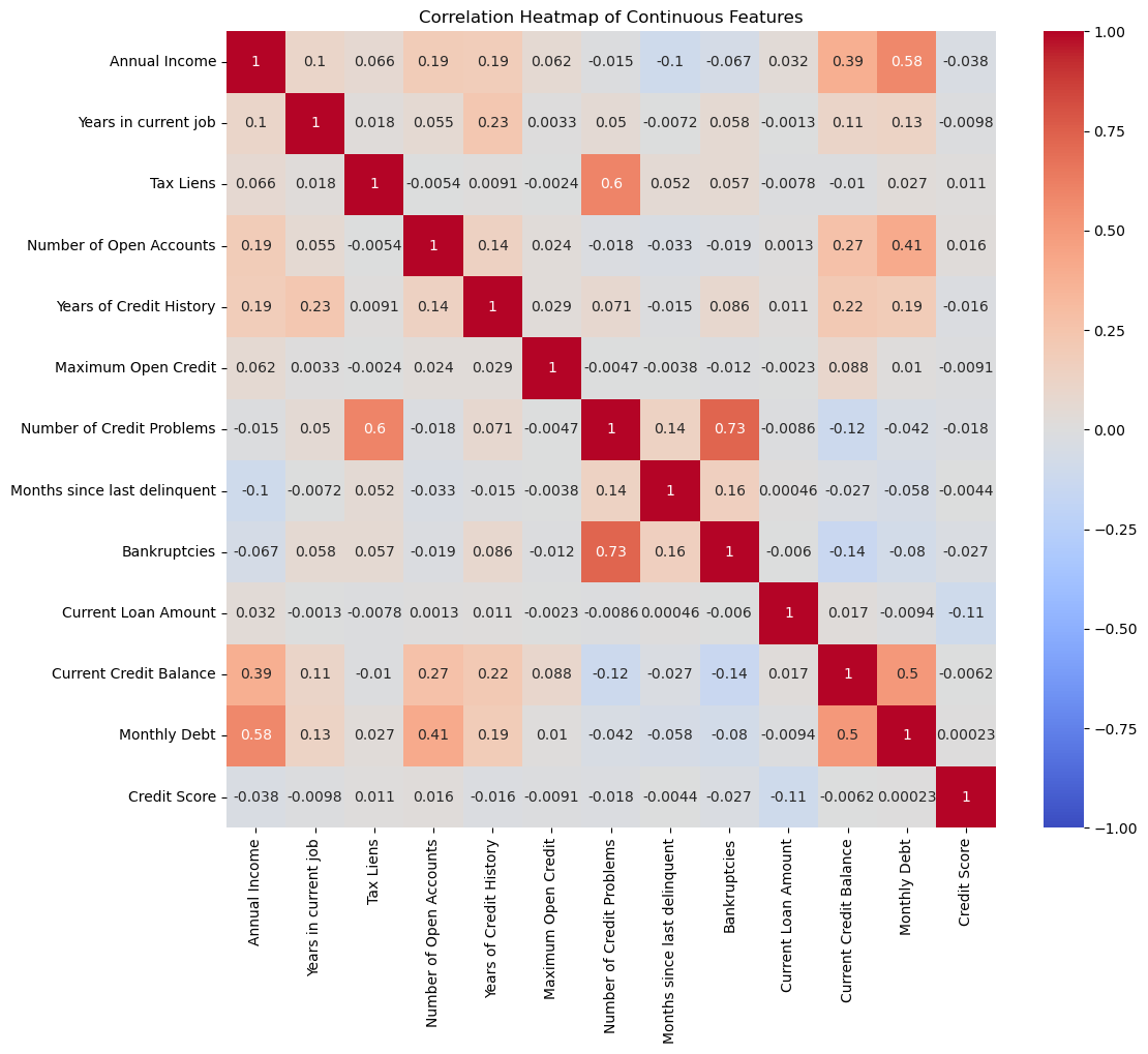
二、绘制热力图
接下来,我们提取数据中的连续值特征,并计算它们之间的相关系数矩阵,最后绘制热力图来展示这些特征之间的相关性。
# 提取连续值特征
continuous_features = ['Annual Income', 'Years in current job', 'Tax Liens','Number of Open Accounts', 'Years of Credit History','Maximum Open Credit', 'Number of Credit Problems','Months since last delinquent', 'Bankruptcies','Current Loan Amount', 'Current Credit Balance', 'Monthly Debt','Credit Score'
]
# 计算相关系数矩阵
correlation_matrix = data[continuous_features].corr()
# 绘制热力图
plt.figure(figsize=(12, 10))
sns.heatmap(correlation_matrix, annot=True, cmap='coolwarm', vmin=-1, vmax=1)
plt.title('Correlation Heatmap of Continuous Features')
plt.show()
需要注意的是,这里的处理比较粗糙,热力图本质上更适合用于连续值的绘制,对于数值型的离散值并不太适用,但为了方便处理,未对数据进行更细致的筛选。
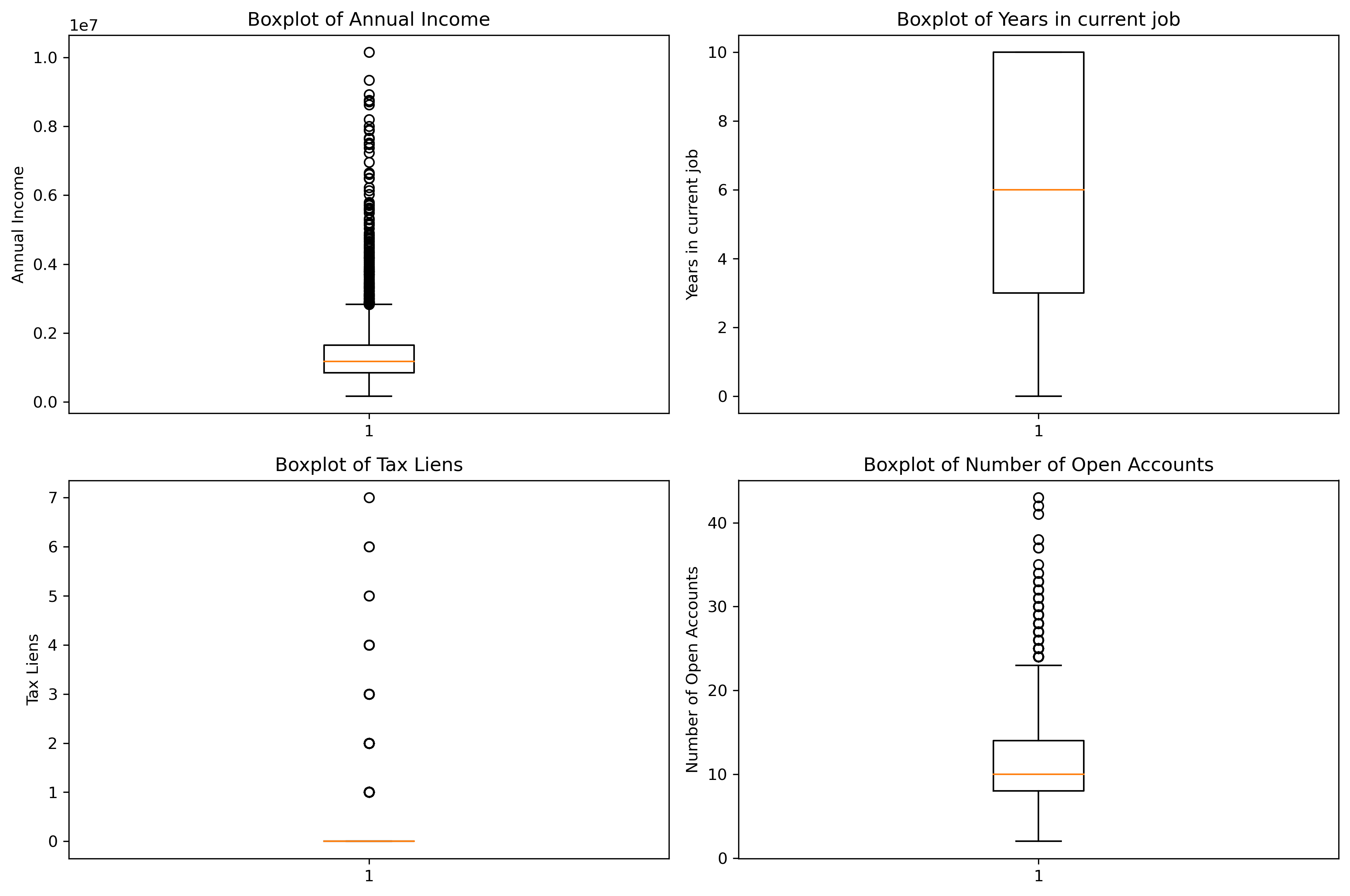
三、绘制子图
我们以绘制箱线图为例,学习如何使用 matplotlib 绘制子图。
3.1 手动指定特征索引绘制子图
# 定义要绘制的特征
features = ['Annual Income', 'Years in current job', 'Tax Liens', 'Number of Open Accounts']# 设置图片清晰度
plt.rcParams['figure.dpi'] = 300# 创建一个包含 2 行 2 列的子图布局
fig, axes = plt.subplots(2, 2, figsize=(12, 8))# 手动指定特征索引进行绘图,仔细观察下这个坐标
i = 0
feature = features[i]
axes[0, 0].boxplot(data[feature].dropna())
axes[0, 0].set_title(f'Boxplot of {feature}')
axes[0, 0].set_ylabel(feature)i = 1
feature = features[i]
axes[0, 1].boxplot(data[feature].dropna())
axes[0, 1].set_title(f'Boxplot of {feature}')
axes[0, 1].set_ylabel(feature)i = 2
feature = features[i]
axes[1, 0].boxplot(data[feature].dropna())
axes[1, 0].set_title(f'Boxplot of {feature}')
axes[1, 0].set_ylabel(feature)i = 3
feature = features[i]
axes[1, 1].boxplot(data[feature].dropna())
axes[1, 1].set_title(f'Boxplot of {feature}')
axes[1, 1].set_ylabel(feature)# 调整子图之间的间距
plt.tight_layout()# 显示图形
plt.show()
3.2 使用循环绘制子图
为了更简洁地实现子图绘制,我们可以使用循环来代替手动指定索引的方式:
# 定义要绘制的特征
features = ['Annual Income', 'Years in current job', 'Tax Liens', 'Number of Open Accounts']# 设置图片清晰度
plt.rcParams['figure.dpi'] = 300# 创建一个包含 2 行 2 列的子图布局
fig, axes = plt.subplots(2, 2, figsize=(12, 8))# 使用 for 循环遍历特征
for i in range(len(features)):row = i // 2 # 计算当前特征在子图中的行索引,// 是整除,即取整 ,之所以用整除是因为我们要的是行数# 例如 0//2=0, 1//2=0, 2//2=1, 3//2=1col = i % 2 # 计算当前特征在子图中的列索引,% 是取余,即取模# 例如 0%2=0, 1%2=1, 2%2=0, 3%2=1# 绘制箱线图feature = features[i]axes[row, col].boxplot(data[feature].dropna())axes[row, col].set_title(f'Boxplot of {feature}')axes[row, col].set_ylabel(feature)# 调整子图之间的间距
plt.tight_layout()# 显示图形
plt.show()
四、实用函数 enumerate
最后介绍一个非常实用的函数 enumerate,它返回一个迭代对象,该对象包含索引和值。
函数语法:enumerate(iterable, start=0)
参数说明:
iterable:迭代对象,可以是列表、元组、字典、字符串等。start:索引的开始值,默认为 0。
返回值:返回一个迭代对象,包含索引和值。
enumerate 函数的作用在于允许我们同时迭代一个序列,并获取每个元素的索引和值,示例如下:
features = ['Annual Income', 'Years in current job', 'Tax Liens', 'Number of Open Accounts']for i, feature in enumerate(features):print(f"索引 {i} 对应的特征是: {feature}")
输出结果:
索引 0 对应的特征是: Annual Income
索引 1 对应的特征是: Years in current job
索引 2 对应的特征是: Tax Liens
索引 3 对应的特征是: Number of Open Accounts
![]()
通过以上步骤,我们完成了热力图和子图的绘制,并介绍了实用函数 enumerate。
@浙大疏锦行